1. Introduction

The statistical analysis, machine learning, artificial intelligence, database techniques and pattern recognition concepts have magnified the origin of Data mining. Traditional techniques may be inapt due to enormity of data, high dimensionality of data, heterogeneous and dispersed nature of data. In this era, data mining is prevalent in the field of commerce, trade, science, architecture, education and medication fair to remark a few. The area of data mining applications we come across are the mining of genome sequencing, market exchange, clinical experiments and in the transactions of credit card. With the immense of devices gifted of accumulating data, Big data is now used more widely with the collection of data attractively and cheaply.

Frauds existing in tax return, claims of insurances, usage of cell phones, credit card transactions etc. represent substantial problems for corporate and the government but spotting and foiling fraud is not so modest task. Frauds are claimed to be an

adaptive crime, so it desires distinct means of intellectual data mining algorithms which are coming raised in the field of investigation to sense and prevent fraud. These are methods that exist in the areas of machine learning, statistical analysis and knowledge discovery databases. These methods in different zones of fraud crimes do offer appropriate and fruitful solutions.

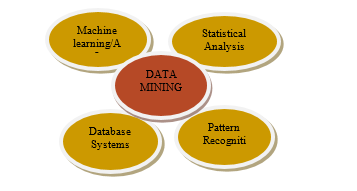Figure 1. Applications of Data Mining.

There are mainly two procedures used for fraud detection statistical performances and artificial intelligence.  Fraud supervision is a knowledge-intensive activity. The main AI Techniques used in the analysis of detecting fraud management include:

• Data mining is the process where facts are classified, clustered and segmented and connotations and instructions in the agreed data are mechanically found that may indicate stimulating patterns, together with those correlated to fraud.
• Expert systems will help to scramble know-how to perceive scam in the way of rules.
• Pattern recognition sense estimated patterns, classes or clusters of mistrustful deeds either routinely or to match assumed inputs.
• Machine learning methods to mechanically find features of frauds.
• Neural networks learn doubtful patterns from samples and used advanced to detect them.

Other techniques such as Bayesian networks, Link analysis, Decision trees and sequence matching are also used for fraud detection.

In field of data mining and knowledge discovery, to handle the problems it is mainly classified into two types supervised learning and un-supervised learning respectively. Supervised learning is further sub-classified depending on the properties of the response variable into classification and regression methods. If the response variable is categorical and discrete, it is classification problems. Otherwise, if the response variable is continuous, it is regression problems. There are different Classification methods for detecting fraud from large data transactions. Selecting Random Forest, Support Vector Machine, Logistic regression and K-Nearest Neighbors [1], our previous work of comparative analysis of these algorithms detected Random Forest to be the best having high accuracy to detect fraud from credit card transactions/ATM card transactions [1].

In this paper, we have given an introduction to Random Forest in section II, description of smote sampling model in section III, about ROSE function in section IV, Theoretical description in section V, proposed algorithm in section VI, followed by Conclusion and References.

2. Introduction to Random Forest

Random Forest can be used to resolve regression as well as classification problems. The dependent attribute or variable is continuous in regression and in classification problems it is categorical. Random Forest is a very influential ensembling machine learning algorithm in which decision tree works as the base classifiers, forming multiple decision trees and then merging the output generated by each of them. Decision tree is a classification model in which it classifies each node with maximum information gain.  This search is continued until all the nodes are beat or there is no more information to gain. Decision trees are very modest and informal to know models; however, their predictive power is less, thus called as weak learners [1].

Random Forest works as an ensemble of random trees. It syndicates the yield of multiple random trees and then to originate up with its own output. Random Forest as similar to Decision Tress [1] but will not select all the data points and variables in each of the trees. It arbitrarily assembles data points and variables in each of the tree that it produces and then it is united to arrive at the output at the end. It takes away the prejudice that was encountered in a decision tree model. Also, it improves the predictive power significantly [2].

Random forest stays a tree-based algorithm which take in building several trees (decision trees), were the manipulator generates the number of trees. The elective of all created trees fixes final classifying outcome.

3. Smote Sampling Method

  Stereotypically, there are several classification problems that have been anticipated to organize formerly disregarded observations, which will be situated, or recognized set to be tested by application of a classifier is then trained by earlier prearranged observations called training dataset. Numerous typical classifiers are anticipated to deal with this type of snags such as tree-based classifiers, discriminant analysis and logistic regression.

Unbalanced data cause problems in many of the learning algorithms. This is due to irregular quantity of cases that is posed by each class of the problem. Synthetic Minority Over-Sampling Technique algorithm (SMOTE) is used for handling these unbalanced classification problems.

The Smote function can be called as defined, when it discourses the unbalanced problems with the creation of a new smote data set. Alternatively, it returns the ensuing model by routing a classification algorithm on the new data set [3].

Smote (form, data, perc. over = 200, k = 5, perc. under = 200, learner = NULL, …)

Definition of the arguments-

Form designates the prediction problem. Data holds the actual unbalanced dataset. Perc. Over is method of over-sampling that finds a figure that initiatives the verdict of how many further cases from the minority class are generated. Perc. Under is an under-sampling where among each case made from the minority class, it specifies an amount that initiate the choice of the number of further cases from the majority classes are designated [4,5]. K is a quantity signifying the number of adjoining neighbors that is further used to produce the new instances of the minority class. Learner is set to Null by default. It acts as a string with a tag of a function that outfits a classification procedure that will be useful in the ensuing smote data set.

The two important constraints that switch the quantity of over-sampling of the minority class and under-sampling of majority class are perc. Over and perc. Under respectively.  Perc. Over will approximately a numeral above 100, thereby perc. Over/100 innovative samples of this class are considered for the minority class. If perc. Over value is below 100 then for an arbitrarily selected proportion of the cases, a single case is created and fit into the minority class on the original dataset. The perc. Under constraint panels part of the cases of majority class that erratically selected as the final balanced dataset. With respect to the count of newly engendered minority class cases, the result is obtained [3], [5].

Designed for each existing minority class, ‘n’ new-fangled instances will be formed which is measured by the parameter perc. Over. The instances will be generated by using the parameter K that holds the count of neighbours [3], [6].

We arrive directly to the classification model from the resulting balanced dataset by using the above-mentioned function [5]. Overall, this function will either return Null value or a new dataset depending on the usage of smote function. If not, the learner parameter will return the classification model [5].

4. Rose: A Package for Binary Imbalanced Dataset

Imbalanced learning signifies the problematic of supervised classification if a class behave erratically over the sample dataset. The Rose, Random Over Sampling Example [7] tackles these problems with its on functions embedded in the package. The class imbalance circumstances are persistent in the multiplicity of applications and fields; this issue had received considerable attention recently [8]. There originate the scarcity of software and procedures clearly meant to handle imbalanced data so to have the non-expert users adopt it. In the R environment, there exist Caret package to validate as well as select classification and regression complications. It highlights the issue of imbalance class as down-sample and up-sample [6][8]. It is worth indicating DMwR (Torgo,2010) which gives an estimation of any classifier, thereby handles imbalanced learning.

The ROSE package was motivated to enhance the performance of an imbalanced setting of binary classification providing both standard and more refined tools [7]. Menardi and Torelli at 2014 had developed the smoothed bootstrap-based method. By aiding the phases of model estimation and assessment ROSE [7] relieved the gravity of the effects of an unbalanced distribution of classes.

5. Theoretical Background

5.1. Ensemble Classifiers

An ensemble contains a set of independently trained classifiers whose predictions are combined for categorizing new instances [2].

Bagging [9] and Boosting (Robert E Schapire,2003) are two popular methods for producing ensembles. Bootstrap gathering samples stands for the process called Bagging. As portion of ensemble, if “n” individual classifiers are to be produced from a given original dataset of size “m” then n distinct training set of size m is engendered using sampling. In bagging multiple classifiers created are not dependent on each other. In boosting, from the training dataset each sample is allotted weights. The classifiers generated by boosting is dependent on each other.

• Definition of Random Forest

Random Forest classifier comprise group of tree-structured classifiers t(x, Ɵ_n ) n=1,2…. , where the Ɵ _n  are self-regulating identical scattered random vectors and every tree casts a unit vote for the most popular class at input x, [2][10].

 Once the forest is trained or constructed, each tree give rise to new instance which is recorded as vectors and is joined. The new instance is taken by considering the class having the maximum votes. Nearly one-third of original instances are left, after sampling with replacement of every tree the bootstrap sample set is drawn. The new instances obtained is the out of bag (OOB) data. Out-of-bag error estimation is calculated considering every individual tree’s OOB dataset in the forest.

Illustrating Accuracy of Random Forest:

The Generalization error (Pe^*) of Random Forest is Use “(1)”,

 where mg (X, Y) is margin function. The margin function measures the level to which the average count of votes at the point (x, y) for the exact class surpasses the average votes of any further class. Here x is the predictor vector and y is the classification.

The Margin function is Use “(2)”,

Here, I is the indicator function.

Boundary is directly proportional to confidence in the classification.

Benefit of Random Forest is specified in terms of the predictable value of Margin function Use“(3)”.

A function of mean correlation amongst base classifiers and average strength results in the generalization error of ensemble classifier (Prenger. R, et al,2010). If the mean value of correlation is low an upper bound for generalization error is Use“(4)”,

6. Aggrandized Random Forest.

 For this work, we have used large dataset of about three lacs of credit card transactions. The classification algorithm is built in the R platform. The proposed algorithm is named Aggrandized Random Forest, which have an increase in its accuracy by 3.06 % for balanced data and an increase of 3.30% for imbalanced data, compared to the previous work as shown in Table.2.

Aggrandized Random Forest is proposed by considering the random forest as the base classifiers with bagging approach and compared with the existing random forest. It is analyzed that Bagged Random Forest gives better results.

 Here, we have used the ROSE package of R, to train the imbalanced data set. The functions in ROSE [7,8] have improved the capacity of generalization and reduced the risk conceded by other oversampling methods. As will be expounded, the ROSE technique can be truly considered, which reduces the repetition of instances. In accuracy evaluation step, the overall accuracy may yield misleading results, thus the aggrandized random forest has been evaluated in rapports of class -independent extents such as precision, recall, F-measures etc., as mentioned in the Table.1.

The required library functions in R,

library(caret)

library(caTools)

library (ROSE)

library (random Forest)

6.1.  The Usage of ROSE Function:

ROSE (formula, data, N, subset = options(“subset”) $subset, seed)

Defining the arguments:

Formula represents the object of class formula where the class label representing the route is allotted with a sequence of routes thru the predictors. The interaction among predictors or their transformations is mentioned by a message. Data argument when not specified the variables are taken from environment. It is an optional argument. N indicates the anticipated trial proportions of the ensuing dataset. By default, the length of the response variable in formula is considered. Seed argument is assigned a single integer value to indicate seeds and preserve the trace of the produced sample [7].

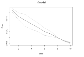Figure 2(a). Represents the rf. model on Balanced Data

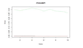Figure 2(b). Represents the rf. Model on unbalanced data.

6.2. Coding for Imbalanced to Balanced Dataset

###imbalanced classification

creditcard$Class<- as. factor(creditcard$Class)

table (is.na (credit card)) ##-is.na-indicates missing elements.

creditcard$Time

str (credit card)

###

split<-sample. split (creditcard$Class, Split Ratio = 0.7)

train<-subset (credit card, split==T)

test<-subset (credit card, split==F)

###removing unbalanced classification problem and making data balanced

train. rose <- ROSE (Class ~., data = train, seed = 1) $data

table (train. rose$Class)

test.rose <- ROSE(Class ~ ., data = test, seed = 1)$data

table(test.rose$Class)

####Applying random forest on Balanced data

rf.model<-randomForest(Class~., data = train.rose ,ntree=10)

rf.model “As in Figure.2(a)”.

####Applying random forest on unbalanced data####

rf.model1<-randomForest(Class~., data = train ,ntree=10)

rf.predict1<-predict(rf.model1,newdata = test)

plot(rf.model1) as plotted “As in Fig.2(b)”.

6.3. Confusion Matrix.

After the performance of a classifier, we can engender confusion matrix grounded on the prediction results where each column of the matrix represents the instances in a predicted class, while each row represents the instances in an actual class.

The table consists of two rows and columns that gives the count of true positives (TP), false positives (FP), true negatives (TN) and false negatives (FN). The minority class is the positive class and the majority class is the negative class “As in Figure.3”.

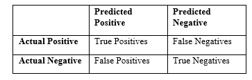Figure 3. Confusion matrix representation.

6.3.1 The Confusion Matrix for The Proposed Algorithm.

Confusion matrix to evaluate OOB error rate “As shown in Figure.4”.

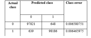Figure 4. OOB estimate of error rate: 0.65%.

6.3.2. Confusion matrix for balanced dataset and imbalanced dataset

The “Figure 5 (a)” represents the confusion matrix for the balanced dataset, and “Figure 5 (b)” represents the confusion matrix for imbalanced dataset, where we could get true positive value, false positive, false negative and true negative value to calculate the parameters precision, recall, f-measure, sensitivity and specificity. Thereafter, the analytical measures are calculated accordingly. 

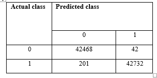Figure 5(a). For balanced data.

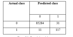Figure 5(b). For unbalanced data.

6.4. Analytical Measures Used for Comparing the Proposed and Existing.

There are several factors which is used to the detect the best performance of the algorithm. The presentation of the proposed system is evaluated using the analytical measures such as precision, recall, f-measure etc. [1]

• Precision = TP/(TP+FP)
• Recall = TP/TP+FN)
• F-Measure = 2 *(precision * recall) / (precision + recall)
• Sensitivity= TP/FP
• Specificity=TN/FN

Along with the above-mentioned factors, the other evaluated factors are Accuracy, Kappa, prevalence, detection rate, detection prevalence, P -value, Positive Pred. value, Negative Pred. value, Mcnemar’s Test P- Value, AUC etc.

Precision measured by the count of true positives divided by the sum of true positives and false positives.

Recall measures the figure of the true positives divided by the sum of true positives and false negatives.

The F-Measure indicates the stability between precision and recall values.

Kappa statistics characterize the range to which the data is collected correctly.

Sensitivity refers to the comparison of the count of acceptably recognized as fraud to the amount incorrectly listed as fraud. It is the ratio of true positives to false positives.

Area Under the Curve (AUC) is used to analyze the performance of classification models capable to predict the classes accurately [11,12].

Detection rate is mainly reflected in confusion matrix. This parameter will vary according to the   dataset.

Detection rate=TP/(TP+FP+FN+TN).

Specificity indicates the same concept with genuine transactions, or the assessment of true negatives to false negatives.

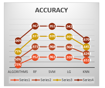Figure 6. Accuracy of the comparative study of previous work for detecting 100% fraud in the dataset [1].

The previous work was a comparative study of different classification algorithms such as Random Forest [12-15], SVM, K-nearest neighbor and Logistic Regression [1] to detect fraud from credit card transaction. It was found that the Random Forest Algorithm [15] is best in detecting the fraud with an accuracy of 0.9675 “As shown in Figure.6”.

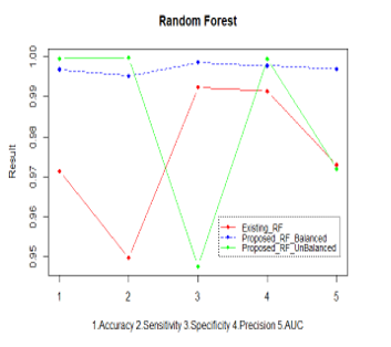Figure 7. Performance of the proposed Random Forest

Table 1. Comparison of Analytical Measures for the Aggrandized Random Forest Results with Those of the Existing Random Forest.

Factors	Existing Random Forest	For Balanced Dataset	Imbalanced Dataset
Accuracy	0.9675	0.9972	0.9995
95% CI	0.9562, 0.9766	0.9968, 0.9975	0.9993, 0.9996
No Information Rate	0.5182	0.5006	0.9983
P-Value	< 2.2e-16	< 2.2e-16	< 2e-16
Kappa	0.9348	0.9943	0.8476
Mcnemar’s Test P-Value	5.806e-07	< 2.2e-16	0.00337
Sensitivity	0.9391	0.9953	0.9999
Specificity	0.9939	0.9990	0.7905
Pos. Predc Value	0.9930	0.9990	0.9996
Neg. Predc Value	0.9461	0.9953	0.9141
Prevalence	0.4818	0.4994	0.9983
Detection Rate	0.4525	0.4970	0.9981
Detection Prevalence	0.4556	0.4975	0.9985
Balanced Accuracy	0.9665	0.9972	0.8952
‘Positive’ Class	Yes	0	0
AUC	0.970	0.997	0.957
Precision	0.9915	0.9978	0.9995
F-measure	0.9645	0.9965	0.9996

The comparison of the Aggrandized Random Forest with the existing Random Forest “As shown in Figure.7”. The analytical measures considered to detect the performance of the new proposed random forest; Aggrandized Random Forest “As shown in the Table 1”.

The Analytical measures for the Proposed and the existing is represented by chart diagram “As in Figure.8”. The ROC curve which is the receiver operating characteristics of the proposed Random Forest “As shown in Figure 9(a) and Figure 9(b)” for the balanced and imbalanced dataset respectively.

Table 2. Performance of Aggrandized RF.

Dataset	Accuracy	Sensitivity	Specificity	AUC	Precision	Kappa	F-Measure
Existing RF	0.9675	0.9391	0.9939	0.970	0.9915	0.9348	0.9645
Proposed RF Balanced	0.9972	0.9953	0.9990	0.997	0.9978	0.9943	0.9965
Improvement (%)	3.06	5.98	0.51	2.78	0.63	6.36	3.31
Proposed RF Imbalanced	0.9995	0.9999	0.7905	0.957	0.9995	0.8476	0.9996
Improvement (%)	3.30	6.47	-20.46	-1.34	0.80	-9.32	3.63

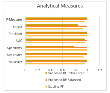Figure 8. Chart Diagram signifying the comparative recital of Aggrandized Random Forest with Balanced and Imbalanced Dataset to the existing Random Forest Algorithm.

The overall performance of the Aggrandized Random Forest with balanced and imbalanced dataset is evaluated with the existing random Forest, and found to have more accuracy, sensitivity, F-measure, precision, etc. The Table 2 gives the improvement of the proposed algorithm.

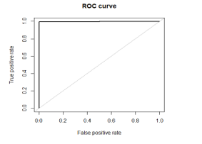Figure 9(a). ROC of balance dataset.

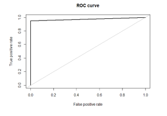Figure 9(b). ROC of imbalanced dataset.

7. Conclusion

In this paper, our proposed algorithm Aggrandized Random Forest is developed in R platform, having a better accuracy of 0.9972 for balanced and 0.9995 for imbalanced data. The results show that for an imbalanced data, Random Forest outstrips other classification techniques and henceforth stays excessive scope for developing improved Random Forest. Using random forest as a base learner can achieve good outcome in the domain of Imbalanced data.

Acknowledgement

We author thank all the contributors of this journal for considering the article. I would like to thank my guide for giving his support and encouragement in my work. Also, thank the authors of the references giving me the privilege to cite their article and enhance my knowledge. With the responsibility as Ph.D. scholar at Nehru arts and science college, I thank all the teachers and my friends in giving their valuable ideas and support. Wish this article will be beneficial for future scholars.

1. M.V. Jisha., D. Vimal Kumar, “An Efficient Credit Card Fraud Classifier of the four data mining classification algorithms- “A Comparative Analysis.”(JETIR)Journal of Emerging Technologies and Innovative Research. Nov.2018, vol 5, issue 11, Pno- 371-378. https://jetir1811656.pdf.
2. Bernard S Heutte L, Adam S, “Dynamic Random forests, Pattern Recognition Letters”, 33 (2012),1580-1586.
3. Tianxiang Gao, “Hybrid classification approach of Smote and instance selection for imbalanced Datasets”. Iowa University, Iowa. Thesis work, 2015.
4. Vrushali Y, Kulkarni, Pradeep K Sinha. Pruning of Random Forest Classifiers: A survey and future directions.”2012 international Conference on Data Science & Engineering (ICDSE), 2012.
5. R Documentation[online]Http://www.rdocumentation.org.
6. Kuhn. caret: Classification and Regression Training,2014. URL http://CRAN.R-Project.org/package=caret.
7. Lunardon, G. Monardo, and N.Torelli, R package ROSE: Random Over Sampling Examples(version0.0-3). Universität di Trieste and Universität di Padova, Italia ,2013.URL http://CRAN.Rproject.org/web/packages/ROSE/inedx.html.[p79][online].
8. ROSE:A package for Binary Imbalanced/Balancing data, Https://journal.r-project.org/archieve/2014-008/RJ-2014-008.pdf.
9. Breiman L, Bagging Predictors, Technical Report No 421, (1994).
10. Breiman L, Random Forests, Machine Learning, 45,5-32, (2001).
11. Vimal Kumar, M.V. Jisha, “Analytical Measures for Detecting Fraud Using Classification Algorithms”. International Journal of Innovative Technology and Creative Engineering (Ijitce), February 2019, vol 9, No.2 636-644. https://ia601504.us.archive.org/19/items/IJITCEFEB19/IJITCE_vol9no202.pdf
12. Bernard s. Heutte L, Adam S Using Random Forest for Handwritten Digit Recognition, International Conference on Document Analysis and Recognition 1043-1047, (2007).
13. Bernard S Heutte L Adam S, Towards a Better Understanding of Random Forests Through the Study of Strength and Correlation, ICIC Proceedings of the Intelligent Computing 5^th International Conference on Emerging Intelligent Computing Technology and Applications, (2009).
14. Bernard S Heutte L Adam S, Forests-RK; A new Random Forests Induction Method, Proceedings of 4^th International Conference on Intelligent Computing: Advanced Intelligent Computing Theories and Applications – with Aspects of Artificial Intelligence, Springer – Ver lag, (2008).
15. Bernard S Heutte L Adam S, On the Selection of Decision Trees in Random Forests, Proceedings of International Joint Conference on Neural Networks, atlanta, Georgia, USA, June 14-19,302-307, (2009).

(Click Here)

(Click Here)