1. Introduction

Emulation consists in replacing a part of the electrical system with another system that has similar characteristics but is more convenient to implement. This technique has become popular in the field of electronic circuits with the (re)introduction of mem elements [1, 2]. For example, the memristors and other promising nanodevices for digital computational systems, massively parallel analog computations or elegant modeling of the neuron cells, are still in the experimental phase and are not available as off-the-shelf components. Emulation allows performing circuit experiments with equivalents of these novel elements and is also useful for demonstration and educational purposes [3].

The first emulators were proposed as analog circuits. Single-purpose emulators such as [4–6] are simple and elegant, but their disadvantage is the inability to change easily their characteristics. Emulators of memristive, memcapacitive and meminductive devices based on mutators provide large universality because they transform a nonlinear resistor, which can be easily modified, to the respective constitution relation of the mem element [7–8].

Another problem is the emulation of blocks with floating ports, which is difficult for purely analog emulators. Several two-terminal floating emulators were proposed [5, 9, 10]. However, all the emulators are based on grounded devices and are “floating” only in the case of neglecting parasitic parameters. In [11], a genuinely floating memcapacitor was proposed on the principle of switched capacitors. The first implementation of a floating resistive port using a mixed-mode system was proposed in [12] with the use of a digital potentiometer, whose resistance was controlled by a microcontroller by means of pre-programmed algorithms.

On the other hand, there are dynamic systems that cannot be emulated via the above single-purpose emulators. For example, the well-known Hodgkin-Huxley model of the cell membranes in a neuron is represented by a set of nonlinear differential equations [13]. The equivalent electrical model is a two-terminal device, consisting of a linear capacitor, two nonlinear memristive devices, and biasing sources [14]. Usually, these models contain large-value inductors and capacitors, which are not useful for practical laboratory experiments.

The demand for emulating general dynamic systems resulted in developing mixed-mode analog-digital emulators [15, 16]. They consist of a central digital unit, which controls one or more floating analog ports of three possible types: controlled voltage source, controlled current source, and digital potentiometer [17]. The independent port currents and voltages are digitally processed according to the mathematical model of the emulated device, and the computed dependent quantities are used for controlling the analog ports. A great advantage of such an approach is the ability to change easily the emulated system by means of changing the software and the possibility of designing truly floating ports with the use of digital isolators without compromising the precision.

The paper summarizes our experience of the emulation of two complex nonlinear dynamic systems via the mixed-mode approach [15]. The problem of discretization analog system and its (in)stability, which occurs when connecting a digital emulator to an analog circuitry, is analyzed. The paper is an extension of our paper [1] presented at the NGCAS 2018 conference in Valletta, Malta. The extended version deals newly with the choice of the integration method and provides a deeper stability analysis and more examples of emulation of biological models.

2. Emulation Principle

2.1.  Basic Setup

In general, the emulator represents a mixed-mode analog-digital system with m floating electrical ports. For the purpose of emulation, let us constrain ourselves to such systems where each port has an independent input quantity (voltage or current) and the other quantity (current or voltage) is computed as a response.

Thus, the emulator consists of a digital core, implemented in a microcontroller (MCU) or FPGA, and ports in the form of controlled current or voltage sources, Figure 1. Using A/D converters with a supporting circuitry, the core measures independent quantities, computes the response, and sets the dependent quantities using D/A converters, followed by reconstruction filters and corresponding controlled sources.

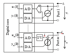Figure 1: Multiport emulator shown with controlled current source at Port 1 and controlled voltage source at Port m.

The emulated system is generally a nonlinear discrete-time system of the n-th order with m inputs and m outputs, whose mathematical representation can be written as

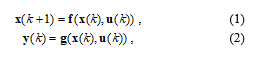where x(k)ÎRⁿ is the state vector, u(k)ÎR^m are the samples of independent (input) quantities, and y(k)ÎR^m are the dependent (output) quantities. The continuous functions f:(Rⁿ,R^m)®Rⁿ and g:(Rⁿ,R^m)®R^m are generally nonlinear.

Figure 2 shows the time characteristics of a discrete-time system (1), (2) implemented in a real logical device and connected to a continuous-time circuit. The inputs u(k) are sampled with a period T and the outputs y(k) are available after the computation and transfer delay t_c < T. The analog circuit the emulator is connected to, which formally includes the anti-aliasing and reconstruction filters, responds to the new outputs y(k), and the response is sampled as the next input u(k+1).

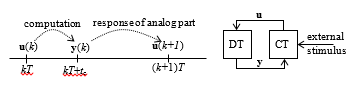Figure 2: Timing of the emulation process (DT – discrete-time emulator, CT – continuous-time analog circuit).

2.2.  Stability of Emulation

As shown in Figure 2, connecting the emulator to an application circuit creates a feedback system, which combines discrete-time and continuous-time parts. Let us consider the one-port case (m = 1). The stability of some fixed point of the system (1), (2) can be examined by linearizing the state description

where AÎR^n´n, BÎR^n´1, CÎR^1´n, and DÎR are real matrices.

Equations (3), (4) represent a single-input single-output linear system, which can be characterized by the z-domain input-output transfer function [18]

where “adj” denotes the adjoint matrix, I is the unity matrix, and U(z) and Y(z) are the z-transforms of the sequences u(k) and y(k).

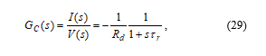
The D/A converter generates a continuous-time signal y(k)®y(t), which stimulates the analog circuit, and the circuit response is sampled by the D/A converter as u(t)®u(k). The continuous-time circuit, which also includes the anti-aliasing and reconstruction filters, can be linearized around an operating point, which corresponds to the fixed point of the discrete system. The input-output small-signal transfer function will be

where U(s) and Y(s) are the Laplace transforms of the continuous-time signals u(t) and y(t).

Considering the signal conversion y(k)®y(t)®G_c®u(t)®u(k), the properties of the analog circuit can also be characterized in the discrete domain by means of the pulse transfer function [18]. For the zero-order hold (ZOH) D/A converter the transfer function will be

where Z{·} denotes the z-transform of the sampled impulse response of the continuous-time transfer function, (1-e^–Ts)/s is the transfer function of ZOH, and  represents the processing delay t_c, which was formally added to the response of the analog circuitry. Note that (7) neglects the quantization introduced by real D/A and A/D converters.

Then the characteristic closed-loop equation will be

The roots of (8) determine the stability of the emulation process.

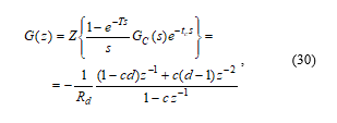
The existence of two types of port (controlled current or voltage source, see Figure 1) is also dictated by the requirement of emulation stability. Let us consider a simple emulation of the resistor R_E by a controlled current source. Then the independent quantity will be the voltage (u ≔ v) and the dependent quantity will be the current (y ≔ i). The emulator transfer function (5) will be simply

i.e. i(k) = v(k)/R_E.

Let the emulator port be loaded with a physical resistor R. Considering a first-order reconstruction filter, but no anti-aliasing filter and no processing delay the small-signal transfer function (6) will be

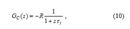where τ_r is the time constant of the reconstruction filter. The positive current i flows into the positive terminal of the emulator port, i.e. (10) has the negative sign.

The pulse transfer function (7) will be

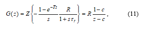where c = exp(-T/τ_r).

Substituting (9) and (11) into the characteristic equation (8) leads to

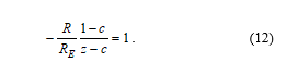Considering the stability condition |z| < 1 for the root of (12) and with respect to the typical choice τ_r » T, which gives 0 < c < 1, we obtain the condition

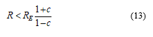for stable operation of the emulating process. Thus, if the Thévenin-equivalent resistance of the analog circuitry connected to the emulator port is higher than the limit (13), the system will oscillate, although the emulated device is a positive-value resistor. A more detailed analysis for other types of devices can be found in [19].

The example underlines the necessity for an emulation-stability analysis. A circuit that would be perfectly stable if realized from physical components may become unstable if some parts are emulated by a discrete-time system.

3. Demonstrations

3.1.  Emulator Hardware

The emulator used for demonstrations is a two-port modification [17] of our emulator [15]. The system consists of the main board STM NUCLEO-F722ZE with a 32-bit MCU ARM Cortex-M7 with a single-precision floating-point unit connected to PC via USB. An add-on card implements two isolated ports, each with 16-bit A/D and D/A converters. The ports are fully floating, which is achieved by the use of integrated DC-DC converters and digital SPI isolators for converter control. The total parasitic capacitance of the floating part to the ground is about 11 pF.

A pluggable controlled voltage or current source can be connected to the ports as shown in Figure 3. The operating area of the four-quadrant voltage and current modules is ±3 V and ±3 mA. The emulator can easily achieve a sampling rate of 100 kHz. Depending on the software, it can emulate one or two independent floating devices or a general two-port network.

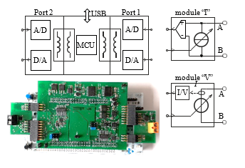Figure 3: Emulator with pluggable IO modules.

3.2.  FitzHugh-Nagumo Model

The FitzHugh-Nagumo (FHN) model of neuronal excitability [20] is a simplification of the well-known Hodgkin-Huxley model [13]. The model represents the prototype of an excitable system. When the input quantity exceeds some certain threshold, the system will generate a pulse. The two-dimensional FHN model is given in its normalized form as

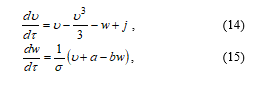where u represents the normalized membrane potential, w is an auxiliary variable, j is a stimulus current, and τ is the model time. The model dynamics is determined by a set of three parameters with the usual values a = 0.7, b = 0.8, and s = 12.5 [21].

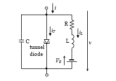Figure 4: Equivalent circuit to (14) and (15) proposed by Nagumo [20].

The system (14), (15) can be represented by an equivalent electrical circuit shown in Figure 4 with a nonlinearity similar to that of the tunnel diode, which was proposed by Nagumo [20]. Let us consider the following mapping of FHN model quantities to the physical circuit in Figure 4:

The transformation coefficients were chosen such that the variable u will represent voltage in volts (k_v = 1 V), j and w will be currents in milliamps (k_i = k_w = 1 mA), and one unit of model time τ will correspond to one millisecond of the physical time (k_t = 1 ms), i.e. the dynamics will be speeded up a thousand times to get a convenient duration of generated pulses.

Considering (16), the parameters of the circuit elements will be

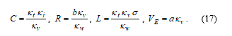For the chosen transformation coefficients we have C = 1 μF, L = 12.5 H, R = 800 Ω, and V_E = 0.7 V. The i–v characteristic i_T(v) of the “tunnel diode” will be

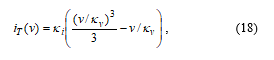which corresponds to the first two terms of RHS of (9).

1) Direct Digital Emulation

Equations (14), (15) represent a dynamical system with the input current j and output potential u. In accordance with the electrical model in Figure 4 the system can be emulated by a controlled voltage source. The output voltage u(k) will be computed from the samples j(k) of the measured current.

The real-time operation of the emulator requires the use of explicit integration methods with low numerical complexity [22]. Let us consider an ordinary differential equation of the n-th order in the form

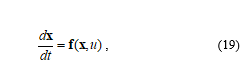where xÎRⁿ and u is a scalar input. Then the explicit multistep linear integration scheme can be formulated as

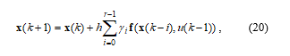where r is the order of the method, h is the integration step, and γ_i are coefficients. For r = 1 we get the classical forward Euler method with γ₁ = 1, and for r = 2 the Adams-Bashforth method of the 2^nd order (AB2) with γ = {3/2, -1/2} [22].

The practical implementation of the multistep scheme (20) has a relative low numerical complexity as it requires just storing r-1 past values f(k–i) := f(x(k–i), u(k–i)).

The computation of each step starts with the evaluation of RHS of (14), (15) for current values of the quantities

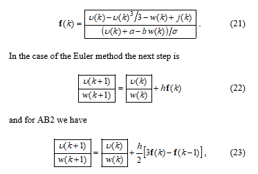where h = T/k_t. The coefficient k_t = 1 ms scales the time axis so that the time unit in the original system (14), (15) corresponds to one millisecond in (22) and (23).

The emulator was configured as a current-controlled voltage source using the module “V”, where the output quantity is the transformed state variable v(k) = u(k) k_v and the control quantity is j(k) = i(k)/k_i. The sampling rate was set to 100 kHz.

Figure 5 shows the results of an experiment where the digital FHN model was “excited” by short pulses with an amplitude of 3 V, a width of 8 ms, and a period of 100 ms applied through a 10 kΩ resistor R_d. It can be seen that each pulse triggers a characteristic excursion, after which the system relaxes back to the equilibrium state.

The discretization and emulation of the continuous-time system bring two problems with the stability: the stability of the integration method itself and the stability of the feedback emulation process as introduced in Section 2.2.

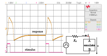Figure 5: Response (channel 1 – orange) to excitation pulses (channel 4 – red).

In particular, it is known for explicit methods that an inappropriate choice of the integration step can lead to instability and an excessive truncation error [22]. Figure 6 shows a qualitative study comparing the performance of the methods (22) and (23) for the same setup as in Figure 5. For the 10 μs sampling period used, the results are indistinguishable from the nominal solution within the uncertainty introduced by the quantization by A/D and D/A converters. When the sampling period was increased to 500 μs, the waveform computed by AB2 showed numerical oscillations. Therefore, the first-order method was preferred in the experiments.

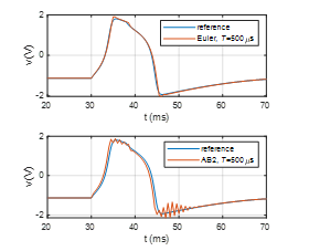Figure 6: Comparison of forward Euler and 2^nd–order Adams-Bashforth methods for large integration steps.

The stability of emulation as introduced in Section 2.2 can be qualitatively assessed based on the equilibrium stability analysis for v = 0, which corresponds to the OFF period of the signal source. The equilibrium of the FHN model can be obtained via solving the system (14), (15) for du/dτ = 0 and dw/dτ = 0, and also by considering the relation v = –R_d i determined by the driving circuit in Figure 5 during the OFF periods. After the transformation (16) the relation becomes u k_v = –R_d j k_i and we obtain the system

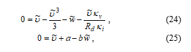
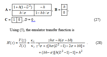
Let us start with the forward Euler method. The equilibrium corresponds to a fixed point of the discretized system (22), because f_k = 0 and thus u(k+1) = u(k), w(k+1) = w(k). The structure of the system (22) corresponds to (1), (2) and its linearization at the fixed point ( , ) leads to the following matrices (3) and (4):

The simulator uses a 1^st-order reconstruction filter with the time constant τ_r and no anti-aliasing filter. The Laplace-domain transfer function between the output of the D/A converter and the input of the A/D converter corresponding to the application schematics in Figure 5 will be

where the negative sign stems from the chosen orientation of v and i.

Using the standard s– and z-transforms, the pulse transfer function can be easily obtained as [23]

where c = exp(-T/τ_r) and d = exp(t_c/τ_r).

The time constant of the reconstruction filter was τ_r = T = 10 μs, which smoothed reasonably its staircase output, and the processing delay was t_c = 3 μs. Then the roots of the characteristic equation (8) are as follows:

λ_1,2 = 0.9978 ± j 0.002289, λ₃ = 0.3692, λ₄ = -3.4988 ´10^-4,

which indicates a stable operation. It can be shown that the doublet λ_1,2 corresponds to the poles of (28) because the FHN model is driven by a high-resistance source, which behaves like a stimulation by a current source (see Figure 5). The doublet is close to the unity circle, reflecting the fact that the sampling rate is orders of magnitudes faster than the modeled dynamics, i.e. the update in each step is relatively low (v(k+1) » v(k)). The roots λ₃ and λ₄ are predominantly influenced by the chosen time constant of the reconstruction filter and MCU processing delay, and represent fast-decaying artifacts of the emulation process.

To compute the z-domain transfer function (5) for higher-order integration methods, the difference equation (20) should be transformed to an equation of the 1^st order.

In the case of the Adams-Bashforth method of the 2^nd order the scheme (23) can be transformed to

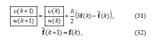where  is the vector of RHS of (14) and (15) delayed by one period. Then the linearization of (31) and (32) leads to

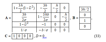Repeating the same procedure as for the Euler method, we obtain the roots:

λ_1,2 = 0.9978 ± j 0.003594,

λ₃ = 0.3681, λ₄ = -0.0136, λ₅ = 0.0130, λ₄ = -3.0454 ´10^-4.

The doublet characterizes the emulated system dynamics and the other roots represent the artifacts of the discretization. Also in this case, the emulation is stable.

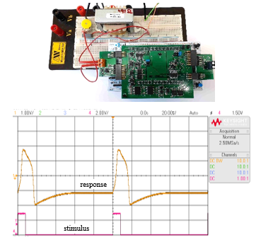Figure 7: Hybrid circuit setup and response (orange) to excitation pulses (red).

2) Hybrid Circuit

In the hybrid approach the emulator is used to implement some parts of the model, while the rest of the model can be realized using standard electronic components as in Figure 4. In the case of the FHN equivalent circuit the emulator implements just the “tunnel diode”. The cubic nonlinearity (18) was emulated as a voltage-controlled current source using the module “I”.

Figure 7 shows the experiment setup on a breadboard and the response of the model for the same conditions as in Figure 5. The parameter L was changed to 16.2 H in this experiment to match the inductance of the available off-the-shelf choke.

Figure 8 compares the measured pulses with a PSpice simulation, the latter being regarded as a reference solution. All three waveforms overlap.

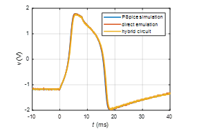Figure 8: Comparison of the measured and simulated responses for L = 16.2 H (all waveforms overlap).

3.3.  Model of Amoeba Adaptation

The amoeba can adapt to periodic environmental changes. An electrical model of the process was presented in [24], see Figure 9. The environmental conditions (temperature and humidity) are represented by a single quantity – the voltage v(t), which is applied to the circuit. The response is the change in amoeba movement velocity represented by the voltage v_c(t).

The memristor in Figure 9 is a voltage-controlled memristor with a threshold whose memristance R_M is governed by the following state equation [24]

confines the memristance between the boundary values R₁ and R₂, and q is the Heaviside step function

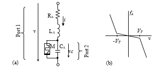Figure 9: (a) Equivalent electrical model of amoeba’s adaptation; (b) Activation function of memristor.

The model leads to a system of the 3^rd order [25]

where the parameters were identified as [24]: R_A = 0.1 Ω, L_A = 2 H, C_A = 1 F, R₁ =3 Ω, R₂ =20 Ω, α = 0.1 Ω/Vs, β = 100 Ω/Vs, V_T = 2.5 V. The amoeba adaptation occurs on the time scale of »100 s, which is rather slow for laboratory experiments even with a digital memory oscilloscope. Therefore the time-axis scaling k_t = 10^-3 was added to the equations. Now, one second of the model time corresponds to one millisecond of the real time.

The emulator was configured as a two-port network. The excitation voltage v(t) is applied to Port 1 with the “I” module (controlled current source). Although the current i(t) is just an internal variable of the system (37)-(39), it can be generated at Port 1 to emulate fully the circuit from Figure 9(a). One ampere in the model corresponds to one milliampere in the emulated circuit. The model response based on v_c(t) is generated at Port 2 with the “V” module. Alternatively, the output can be set as the memristance R_M to monitor the internal state of the model.

Equations (37)-(39) were discretized using the forward Euler method, similar to (22). The window function f_W was realized in the algorithm as a correction of the state variable R_M after each integration step. Whenever R_M > R₂, it is set back to R₂ and vice versa for the lower limit R₁.

The excitation voltage v(t) represents environmental conditions of the amoeba. Favorable conditions correspond to a positive voltage and unfavorable conditions to a negative voltage. Long-term exposure to favorable conditions (v > 0) leads to dR_M/dt < 0 and after a sufficiently long interval the memristance R_M will be at its lower limit, i.e. R_M = R₁.

It has been observed that periodic intervals of unfavorable conditions make the amoeba adapt so that the organism can anticipate the intervals and decrease its velocity. The process can be demonstrated on an experiment from [24]. The “training” voltage waveform consists of three negative cosine pulses

where  is a window function for masking the individual periods of the cosine function. The parameters used were V_F = 0.1 V, V_p = 2 V, and W_p = 5 ms. With respect to the time-axis scaling, the times of pulse starts for the irregular sequence were t_i^(irregular) = {10 ms, 19 ms, 34.5 ms} and for the regular sequence t_i^(regular) = {10 ms, 19 ms, 28 ms}. The excitation signal was generated using the arbitrary waveform generator Keysight 33521B.

The output voltage on Port 2 was generated as [24]

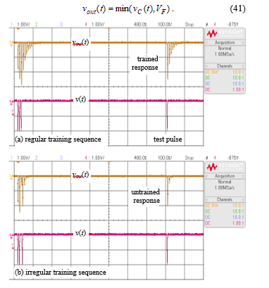Figure 10: Excitation voltage (channel 4 – red) and amoeba response (channel 1 – orange) for (a) regular and (b) irregular training sequence.

Figure 10 shows the excitation voltage v(t) and the response v_out(t) generated by the emulator. The amoeba adaptation is represented in the model by the change of memristance R_M. The application of the irregular sequence of training pulses after a long period of favorable conditions (V_F) does not change the memristance significantly. On the other hand, the regular training sequence makes R_M increase to R₂ and the amoeba becomes “adapted”. Both states can be tested by a single pulse at 800 ms after the training sequence start. The adapted response consists of several pulses of motion slowdown where the organism anticipates other unfavorable intervals. The response of the untrained organism is visibly smaller. Both results are in agreement with computer simulations in [24].

4. Conclusions

The results presented in the paper can be summarized as follows:

(1)    Emulation provides the possibility of substituting an m-port network with a mixed-mode analog-digital system. The network modeled via multi-dimensional differential equations, which link terminal voltages and currents and internal state variables, can be emulated via digitally controlled current or voltage sources. The sources are controlled based on the port voltages or currents and the state variables via discrete-time equations of motion of the system being emulated.

(2)    In some cases, it can be useful to emulate digitally only some key parts of the circuit, while the rest can be made up of (preferably passive) analog components.

(3)    The combination of continuous-time and discrete-time blocks can bring stability problems, even in very simple circuits. The paper presents a methodology that can be used to assess the emulated system stability.

(4)    Stability problems can be alleviated by an appropriate selection of the type of controlled source (voltage or current) which is used to realize each port. Details are given in our previous work [17].

(5)    The paper presents a mixed-mode emulator with pluggable IO ports that has proven itself to emulate unconventional circuit elements (memristors, memcapacitors, meminductors, etc.) and also bio-inspired circuits. Especially in the case of models of biological systems it can avoid using bulky inductors and capacitors, which are common there.

Conflict of Interest

The authors declare no conflict of interest.

Acknowledgment

This work was supported by the Czech Science Foundation under grant No. 18-21608S. The research was also supported by the Project of Specific Research, K217 Department, UD Brno.

1.  Z. Kolka, V. Biolkova, D. Biolek, Z. Biolek, “Hardware Implementation of Bio-Inspired Models” in 2018 New Generation of CAS (NGCAS), Valletta, Malta, 102-105, 2018. https://doi.org/10.1109/NGCAS.2018.8572072
2.  D. Biolek, Memristor emulators. In Memristive networks. Springer book, New York, 2014.
3.  Y. V. Pershin, M. Di Ventra, “Teaching memory circuit elements via experiment-based learning” IEEE Circuits and Systems Magazine, 12(1), 64—74, 2012. https://doi.org/10.1109/MCAS.2011.2181096
4.  Q. Zhaoa, C. Wangb, X. Zhangc, “A universal emulator for memristor, memcapacitor, and meminductor and its chaotic circuit” Chaos 29, 013141, 2019. https://doi.org/10.1063/1.5081076
5.  D.S.Yu, H.Chen, H.H.C.Iu, “Design of a practical memcapacitor emulator without grounded restriction” IEEE Trans Circuits Syst II, 60(6), 207–211, 2013. https://doi.org/10.1109/TCSII.2013.2240879
6.  M.Pd.Sah, R.K.Budhathoki, C.Yang, H.Kim, “Charge Controlled meminductor Emulator” J. of Semiconductor Technology and Science, 14(6), 750–754, 2014. https://dx.doi.org/10.5573/JSTS.2014.14.6.750
7.  D. Biolek, V. Biolková, “Mutator for transforming memristor into memcapacitor” Electronics Letters, 46(21), 1428—1429, 2010. https://doi.org/10.1049/el.2010.2309
8.  D.Yu, Y.Liang, H.H.C.Iu, L.O.Chua, “A universal mutator for transformations among memristor, memcapacitor, and meminductor” IEEE Trans. on Circ Syst Express Briefs, 61(10), 758–762, 2014. https://doi.org/10.1109/TCSII.2014.2345305
9.  Y. V. Pershin, M. Di Ventra, “Emulation of floating memcapacitors and meminductors using current conveyors” Electronics Letters, 47(4), 243—244, 2011. https://doi.org/10.1049/el.2010.7328
10.  M. Kumngern, “A floating memristor emulator circuit using operational transconductance amplifiers” in 2015 IEEE International Conference on Electron Devices and Solid-State Circuits (EDSSC), Singapore, 679–682, 2015. https://doi.org/10.1109/EDSSC.2015.7285207
11.  D. Biolek, V. Biolkova, Z. Kolka, J. Dobes, “Analog Emulator of Genuinely Floating Memcapacitor with Piecewise-Linear Constitutive Relation” Circuits Syst. Signal Process, 35(1), 43-62, 2016. https://doi.org/10.1007/s00034-015-0067-8
12.  Y. V. Pershin, M. Di Ventra, “Practical approach to programmable analog circuits with memristors” IEEE Trans. Circ. Syst. I, 57(8), 1857–1864, 2010. https://doi.org/10.1109/TCSI.2009.2038539
13.  A. L. Hodgkin, A. F. Huxley, “A Quantitative Description of Membrane Current and its Application to Conduction and Excitation in Nerve” J. Physiol., 117(4), 500—544, 1952.
    https://doi.org/10.1113/jphysiol.1952.sp004764
14.  L. Chua, V. Sbitnev, H. Kim, “Hodgkin-Huxley Axon is Made of Memristors” Int. J. of Bifurcation and Chaos, 22(3), 1230011-1-48, 2012. https://doi.org/10.1142/S021812741230011X
15.  D. Biolek, Z. Kolka, J. Vávra, S. Doan, “Universal Emulator of Memristive and Other Two-Terminal Devices” International J. of Unconventional Computing, 12(4), 281—302, 2016.
16.  K. Ochs, E. Solan, S. Dirkmann, T. Mussenbrock, “Wave digital emulation of a double barrier memristive device” in Proceedings of 59th International Midwest Symposium on Circuits and Systems (MWSCAS), Abu Dhabi, 1-4, 2016. https://doi.org/10.1109/MWSCAS.2016.7869946
17.  J. Vavra, Z. Kolka, D. Biolek, “Two-Port Hybrid Emulator of Analog Devices and its Application in Emulation of Memistor” Journal of Advanced Manufacturing Technology (in print).
18.  W.Y. Yang, Signals and Systems with MATLAB. Springer-Verlag Berlin Heidelberg, 2009.
19.  Z. Kolka, V. Biolkova, D. Biolek, “Stability of Digitally Emulated Mem-Elements” in 2015 International Conference on Computing, Communication and Security (ICCCS), Pointe aux Piments, Mauritius, 415—419, 2015. https://doi.org/10.1109/CCCS.2015.7374184
20.  J. Nagumo, S. Arimoto, S. Yoshizawa, “An Active Pulse Transmission Line Simulating Nerve Axon” Proceedings of the IRE, 50(10), 2061—2070, 1962. https://doi.org/10.1109/JRPROC.1962.288235
21.  A. Fuchs, Nonlinear Dynamics in Complex Systems: Theory and Applications for the Life-, Neuro- and Natural Sciences. Springer-Verlag Berlin Heidelberg, 2012.
22.  J. C. Butcher, Numerical Methods for Ordinary Differential Equations, 3rd edition. John Wiley & Sons, Chichester, UK, 2016.
23.  D. Zwillinger, CRC Standard Mathematical Tables and Formulae, 32nd Edition, CRC Press, Boca Raton, 2011.
24.  Y.V. Pershin, S. La Fontaine, M. Di Ventra, “Memristive model of amoeba learning” Physical Review E, 80(2), 021926-1-6, 2010. https://doi.org/10.1103/PhysRevE.80.021926
25.  F. Caravelli, J. Carbajal, “Memristors for the Curious Outsiders” Technologies, 6(4), 118, 2018. https://doi.org/10.3390/technologies6040118

(Click Here)

(Click Here)