1. Introduction

Detection of structural changes in economics has often pose a long standing problem in econometrics [1]. However, most existing tests are designed for structural breaks. Some researchers argued that it’s un-likely that a structural break could be immediate and might seem more reasonable to allow a structural change to take a period of time to take effect. Hence, the technological progress, preference change, and policy switch are some leading driving forces of structural changes that usually exhibit evolutionary changes in the long term.

Structural break examines a shift in the parameters of the model of interest. However, when the conditional relationship between the dependent and explanatory variables contains a structural break, estimates of model coefficients will be inaccurate across different regimes [2]. As such, estimations that do not account for structural breaks will be biased and inconsistent.

        According to [3], one of the traditional methods of detecting structural break is the Chow test analysis. The Chow test  as a method of detecting structural break has the ability of testing for equality of sets of coefficients in two regression models. In this situation, part of the maintained hypothesis of the test is that the error variances will be the same for the two regressions. If this is not the situation, then the Chow test may be misleading and this can result to a situation where by the true size of the test (under the null hypothesis) may not be equal to the prescribed alpha-level. Due to problem like this, the present study will be proposing permutation methods for Chow test analysis for detecting structural break in a linear model.

The permutation test evaluates the probability of getting a value equal to or more extreme than an observed value of a test statistic under a specified null hypothesis. This is achieved by recalculating the test statistic after random shuffling of the data labels. Such tests are computationally intensive and the use of these tests never receive much attention in the natural and behavioral sciences until the emergence of widely accessible fast computer. The basic idea behind permutation methods is to generate a reference distribution by recalculating a statistic for many permutations of the data.

Permutation methods have been found very useful because of their flexibility, distribution-free nature and intuitive formulation, which makes it easy to communicate the general principles of such test procedures to users.

One advantage of the permutation tests over their parametric counterparts is their solid foundations. This is because the validity of the parametric tests relies on random sampling while the permutation tests have their justification on the idea of random allocation of experimental units, with no reference to any underlying population[4, 5].

For researchers in the area of econometrics and users of the traditional Chow test, the most convincing reason to choose the proposed permutation methods for Chow test in determining structural break in linear models is because of the exactness of the p-value obtained using the permutation methods for Chow test instead of the approximated/asymptotic  significant value which is often obtained in other methods. Hence, the permutation method yields a more accurate prediction of how random a given result can be [6-7].

The objectives of this study is to compare the performance of the proposed permutation methods for Chow test analysis against the traditional Chow test and the Milek  permutation method for detecting structural break for the Gamma and Standard Normal distribution.

2. Literature Review

In [8], permutation test was defined as a type of non-parametric randomization test in which the null distribution of a test statistic is estimated by randomly permuting the class labels of the observations.

According to [9], permutation tests for linear model have applications in behavioral studies especially in situations where traditional parametric assumptions about the error term in a linear model are not tenable. In such situations, an improved validity of type I error rates can be achieved with properly constructed permutation tests. More importantly, increased statistical power, improved robustness to effects of outliers, and detection of alternative distributional differences can be achieved by coupling permutation inference with alternative linear model estimators.

In [10], authors explored the framework of permutation-based p-values for assessing the performance of classifiers. Their study examined two simple permutation tests, the first test which assess whether the classifier has found a real class structure in the data where the corresponding null distribution is estimated by permuting the observations in the data and the second test which examines whether the classifier is exploiting the dependency between the features in classification. They observed that the tests can serve to identify descriptive features which can serve as valuable information in improving the classifier performance. The findings of their study revealed that studying the classifier performance through permutation tests is effective. In particular, the restricted permutation test clearly reveals whether the classifier exploits the interdependency between the features in the data.

According [11], permutation test require very few assumptions about the data and can be applied to a wider variety of situations than the parametric counterpart. However, only few of the most common parametric assumptions need to hold for non-parametric test to be valid. The assumptions that are avoided include, the need for normality for the error terms, the need of homoscedasticity and the need for random sampling. With a very basic knowledge of sample properties or of the study design, errors can be treated as exchangeable and/or independent and symmetric and inferences that are not possible with parametric methods can become feasible.

According to [12], permutation tests for structural change from the framework of [13] cannot only be derived for the simple location model but for both the nonparametric and parametric (model-based) permutation tests. Literally, they found that exchangeability of the errors might be a too strong assumption in time series applications where the dependence structure of the observations cannot be fully captured within the model. Although there are time series applications where the errors are not correlated, this assumption impedes the application of permutation methods to many other models of interest.

In [14], author assessed the performance of his permutation for structural break alongside the Chow test, the Nyblom-Hansen test and CUSUM which were all used to detect structural changes in time series. The proposed Milek permutation method was used to detect a trend especially in process control and detection of changes in the average value. The result of the study showed that the proposed method was effective especially in the case of small structural changes.

3. Material and Methods

3.1.  Method of Data Collection

The source of data used for this study were simulation from the Gamma distribution and the Standard Normal distribution for sample size 15, 20, 25, 30, 40, 50, 60, 70, 80, 90 and 100. Secondary data collected from the National Bureau of Statistics and Central Bank of Nigeria (CBN) statistical bulletin on Real GDP and Electricity net generation in Nigeria was used to illustrate the methods. Also, secondary data on monthly reported cases of appendicitis were collected from the records of patients at Federal Hospital Kaura-Namoda, Zamfara State, Nigeria.

3.2. Chow Test

                The Chow test is often used to determine whether there exist different subgroups in a population of interest. The single/full model of a Chow test is written as:

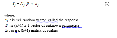
Recall that to estimate the regression parameters  properly using the least-squares estimation, the assumption that n > p holds and X is of full rank. Here n is the number of observation while p is the number of regression coefficients.

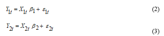
The null hypothesis, tested by Chow, states that two disjoint models with the sum of squares residual is:

where,

and : represents the random variable called the response or dependent variable for the first group and second group respectively.

and : represents constants or parameters whose exact value are not known and thus must be estimated from the experimental data for the first group and second group respectively.

 and : represents the mathematical variable called regressor or covariate or predictor independent non-random variable whose value are controlled or at least accurately observed by the experimenter for the first group and second group respectively.

This suggest that model (2) applies before the break at time t, while model (3) applies after the structural break.

The Chow test asserts that  and with the assumption that the model errors Ԑ_t are independent and identically distributed from a normal distribution with unknown variance [15]. The Chow test basically tests whether the single regression line or the two separate regression lines fit the data best.

Taking advantage of the various F-test [16, 17], to test for presence of structural break in a given set of data, a special and useful application of the F test procedure is found in the Chow test statistic. We must understand that a structural break is when the coefficients of the model change with respect to a time parameter for the Chow test.

Suppose we consider a simple case of (1), that is a simple linear model with one independent variable;

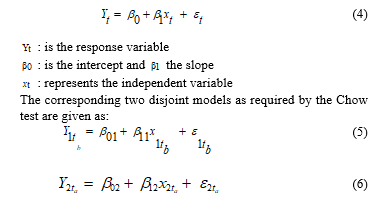
where,

t_a: represents the time at break point and t_b= t_a-1, and : represents the dependent variables for the two disjoint models ( ), and  : represents the intercepts for the two disjoint models ( ), and  : represents the slopes for the two disjoint models ( ),   and  : represents the random error for the two disjoint models ( ), and  and : represents the independent variables for the two disjoint models  ( ).

Recall that the residual sum of squares for the full model can be denoted as RSS_T,

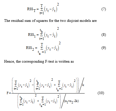Thus, the general Chow test statistics in matrix form is given as

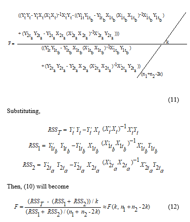where,

RSS_T: represents the residual sum of squares for the full model

RSS₁: represents the residual sum of squares for the first sub sample or first reduced model

RSS₂: represents the residual of the second sub sample or second reduced model,

k: is the number of parameters,

n₁ and n₂: represents the length of the two subsamples.

3.3. Procedure for Running the Chow Test

The stages of running the chow test analysis are as follows:

1. Firstly, run the regression using all the data, before and after the structural break. Collect the sum of squares residual for error RSS_T.
2. Run two separate regression on the data before and after the structural break, collecting the RSS in both cases, giving RSS₁ and RSS₂.
3. Using the three values, calculate the test statistic using (12)
4. Find the critical values in the F-test tables, which has F(k, n₁ + n₂ -2k) degrees of freedom, where k is the number of regressors
5. Take decision and conclude appropriately. The null hypothesis state that there is no structural break against the alternative hypothesis which state that there exist structural break.

Decision Rule

H₀ will be rejected at the significance level α if

The other criterion equivalent to the decision rule above is to compare the p-value for F-statistics with α and reject H₀ if

where P(F) is the asymptotic p-value and note that the rejection of   would mean that  is likely to be different from 0.

A parametric test of significance of the Chow test can be carried out using an F-statistic under the assumption of normality. If this condition is not met, a permutation method becomes an alternative to perform the test. Under normality, one expects a permutation test to produce approximately the same results as the parametric F-test. So, the parametric F-test will be used as a reference to assess some important properties of the various permutation methods proposed in this study.

3.4. The Proposed Permutation Methods for Chow Test

                The proposed permutation methods considered in this study include:

1. Permute object of dependent variable Y_t
2. Permute object of predicted dependent variable

3.4. 1. Method 1: Permute object of dependent variable

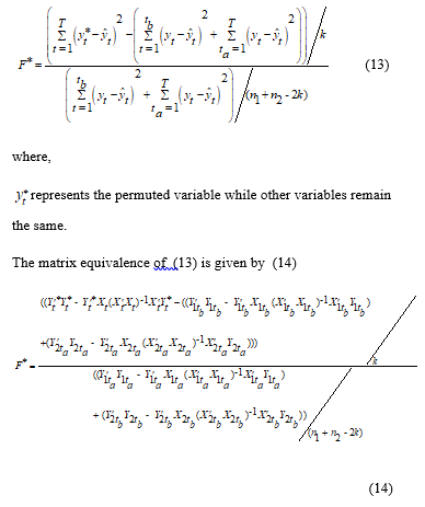
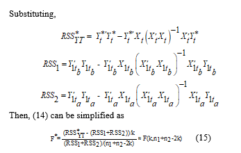
This method considers a situation where we permute the dependent variable  Y_t in (4). For the permutation of  Y_t we shall substitute  to obtain (10) for the simple linear model situation while other variables remain unchanged  represents the permutated dependent variable of the full model) . The F-test statistic for the permutation of the object of dependent variable for the simple linear model is given as

Substituting,

Then, (14) can be simplified as

where,

: represents the permuted residual sum of squares for the full model

: represents the residual of the first sub sample or first reduced model

: represents the residual sum of squares for the second sub sample or second reduced model,

k: is the number of parameters,

n₁ and n₂ : represents the length of the two subsamples

t_a: represents the time at break point and t_b= t_a-1

        The procedure for running the permute the raw data of the dependent variable for the full model Y_t is stated as follows:

1. Compute the sum of squares residual for the single model and the sub sample as RSS_T, RSS₁ and RSS₂. Calculate the reference value of the F-statistic, F using  (12).
2. Permute variable Y_t at random to obtain
3. Compute the sum of squares residual for the single model using and the sub samples to obtain , RSS₁  and RSS₂ as calculated in step 1, compute  using (15).
4. Repeat step 2 and 3 large number of times to obtain the distribution of under permutation. Add the reference value F to the distribution.
5. For a one – tailed test involving the upper tail, calculate the probability as the proportion of values greater than or equal to F. In the lower tail, the probability is the proportion of values smaller than or equal to F.

3.4. 2 Method 2: Permute object of the predicted dependent variable

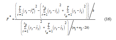
This method considers permuting the predicted dependent variable of the full model.  In this method, the object of the predicted variable will be permuted and used to obtain the corresponding residual sum of squares. We shall express this method using the simple linear model before generalizing using the matrix form.  The F-test statistic for the permutation of the object of predicted dependent variable for the simple linear model is given as

where,

: represents the permuted predicted variable while other variables remain the same.

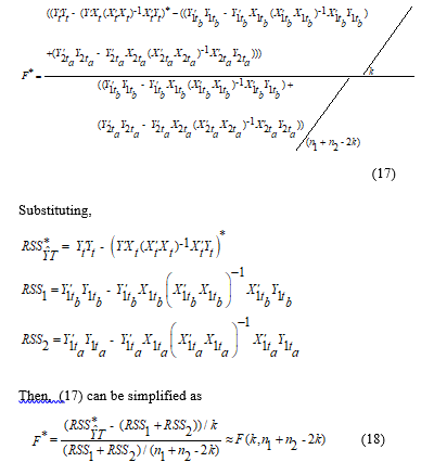
The matrix equivalence of  (16) is given by  (17)

where,

: represents the permuted predicted residual sum of squares for the full model

: represents the residual of the first sub sample or first reduced model

 represents the residual sum of squares for the second sub sample or second reduced model,

k: is the number of parameters,

n₁ and n₂: represents the length of the two subsamples

t_a: represents the time at break point and t_b= t_a-1

The procedure for running the permute the predicted dependent variable for the full model  is stated as follows:

1. Compute the sum of squares residual for the single model and the sub sample as RSS_T, RSS₁ and RSS₂.. Calculate the reference value of the F-statistic, F using (12).
2. Permute variable at random to obtain
3. Compute the sum of squares residual for the single model using and the sub samples to obtain , RSS₁  and RSS₂ as calculated in step 1, compute   using  (18).
4. Repeat step 2 and 3 large number of times to obtain the distribution of under permutation. Add the reference value F to the distribution.
5. For a one – tailed test involving the upper tail, calculate the probability as the proportion of values greater than or equal to F. In the lower tail, the probability is the proportion of values smaller than or equal to F.

3.5.   Milek (2015) Permutation Method for Structural Break

        In [14], the author proposed a permutation method for structural break as

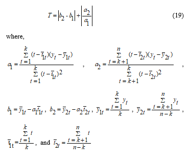The testing procedure for the permutation test to detect a structural change at time t = k is as follows as described by [14] , was presented as:

1. Establishment of the level of significance α
2. Calculate the T₀ value of statistic T based on simulated data.
3. Executing the time series permutations of N times, then calculating the value of the test statistics.
4. On the basis of the empirical distribution of the test statistics T, the asymptotic significance level (ASL) value is calculated. If ASL < α, then the hypothesis H0 is rejected, otherwise there is no basis to reject H₀. As the number of repetitions of permutations assumed N = 1000.

3.6.  Power performance of the Methods

                To determine the power of the methods in this study, data were simulated from the gamma distribution and the standard normal distribution.  The null hypothesis was stated as:

H₀: There is no presence of structural break in the model or

The power of the methods were examined using  the following criteria:

1. The size of the samples n={15, 20, 25, 30, 40, 50, 60, 70, 80, 90, 100}
2. The break points were varied randomly to avoid bias
3. The significant level (α) was set at 95%
4. The permutation was set at 10, 000 permutations

The power was reported as the rate (fraction) of rejection of the null hypothesis after 200 simulations.

The value of power is expected to fall between zero and one ( ), and the decision rule is: the more closely the value of the power is to one, the better the method [18]. Hence, the method with its power more closely to 1 becomes the best method for detecting structural break.

Also, the average power of the methods were calculated as:

where the number of sample size points, S= 1, 2, …, 11

Also, simple bar chart was used to express the visualization of the average power of the methods, where the method with the highest bar is considered the best method. Thereby, the height of the bar determines the magnitude or performance of the methods.

3.7.   Data Presentation

Table 1: Summary of Annual Real Gross Domestic Product and Electricity Net Generation from 1989-2015

Year	RGDP(“B” N)	ENG (“B” kwh)	Year	RGDP (“B” N)	ENG (“B” kwh)
1989	236.7	12.251	2003	477.5	19.352
1990	267.5	12.029	2004	527.6	23.171
1991	265.4	13.613	2005	561.9	22.524
1992	271.4	14.247	2006	595.8	22.109
1993	274.8	13.913	2007	634.3	21.922
1994	275.5	14.877	2008	672.2	22.680
1995	281.4	13.889	2009	716.9	22.879
1996	293.7	14.367	2010	775.3	23.143
1997	302	14.697	2011	884	27.522
1998	310.9	14.732	2012	888.9	29.240
1999	312.2	15.432	2013	950.1	29.538
2000	329.2	14.131	2014	955.2	29.697
2001	357	14.837	2015	536.68	34.65
2002	433.2	19.953

Source: Central Bank of Nigeria Statistical Bulletin and National Bureau of Statistics Annual Abstract of Statistics for various years

Key: RGDP = Real Gross Domestic Product in billions of Naira and ENG=Electricity Net Generation in billion Kilo Watt per hour

Table 2: Number of Monthly Reported Appendicitis cases for the period of 2011 to 2017

MONTHS	YEARS
	2011	2012	2013	2014	2015	2016	2017
January	7	8	4	8	5	4	2
February	4	6	5	6	4	3	3
March	7	8	3	4	3	2	1
April	9	4	6	5	2	4	2
May	5	9	4	4	4	5	1
June	3	7	5	2	5	0	1
July	9	9	1	7	5	3	1
August	6	9	4	5	3	5	3
September	7	7	5	5	0	3	2
October	6	5	6	4	5	1	3
November	9	8	7	7	4	2	2
December	6	4	6	3	6	3	1
Total	78	84	56	60	46	35	22

Source: Federal Hospital Kaura-Namoda, Zamfara State, Nigeria, 2018

4. Data Analysis and Result

                In this section, the result of simulation was obtained for the various methods discussed in the previous section. Also, result of the real life application of the methods were equally presented in this section. The data analysis was done using computer program written in R.

4.1.    Result of Data Analysis for  Gamma Distribution

This section presents the power of the various methods using data generated from the gamma distribution at α=0.05.

Table 3: Performance of the methods for  Gamma Distribution

Sample Size / Methods	Chow	Method1	Method2	Milek (2015)
15	0.42	0.8	0.56	0.04
20	0.44	0.84	0.56	0.04
25	0.68	0.9	0.58	0.04
30	0.7	0.9	0.66	0.06
40	0.82	0.94	0.72	0.06
50	0.84	0.96	0.82	0.06
60	0.84	0.96	0.86	0.06
70	0.9	0.96	0.88	0.08
80	0.9	0.96	0.88	0.08
90	0.94	0.96	0.88	0.08
100	0.94	0.97	0.9	0.14
Average Power	0.77	0.92	0.75	0.07
Rank	2	1	3	4

 4.2.   Result of Data Analysis for  Standard Normal Distribution

This section presents the power of the various methods using data generated from the standard normal distribution at  α=0.05.

Table 4: Performance of the methods for  Standard Normal Distribution

Sample Size / Methods	Chow	Method1	Method2	Milek (2015)
15	0.56	0.92	0.52	0.2
20	0.56	0.92	0.52	0.2
25	0.58	0.92	0.54	0.2
30	0.58	0.92	0.54	0.2
40	0.6	0.94	0.56	0.2
50	0.6	0.94	0.56	0.2
60	0.58	0.94	0.86	0.28
70	0.7	0.95	0.86	0.6
80	0.7	0.96	0.88	0.8
90	0.73	0.98	0.88	0.8
100	0.74	0.98	0.88	0.8
Average Power	0.63	0.94	0.69	0.41
Rank	3	1	2	4

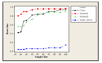Figure 1: Performance of the methods for the Gamma Distribution

Table 5: Performance of the methods across the Distributions

Methods	Gamma Distribution	Standard Normal Distribution	Average Power for all distribution	Rank
Chow	0.77	0.63	0.70	3
Method1	0.92	0.94	0.93	1
Method2	0.75	0.69	0.72	2
Milek (2015)	0.07	0.41	0.24	4

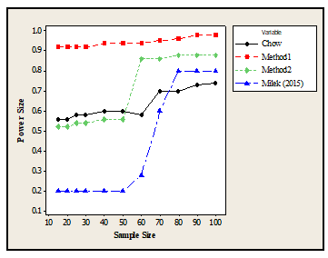Figure 2: Performance of the methods for the Standard Normal Distribution

4.3.  Discussion of Result

The result of the analysis presented in table 3 using data for the gamma distribution showed that Method1 performed best in terms of rejecting the null hypothesis when it is true at 95% Confidence level while the least performing method was the Milek, since their corresponding performance/rank were obtained as Method1 = 1, Chow= 2, Method2=3  and Milek (2015) =4. The findings was presented in figure 1 and it was revealed that the performance of the methods increases as the sample size increases.

Similarly, it was found from the result presented in table 4 for the standard normal distribution that Method1 performed best in terms of rejecting the null hypothesis when it is true at 95% Confidence level while the least performing method was the Milek, since their corresponding performance/rank were obtained as Method1 = 1, Method2 = 2, Chow=3  and Milek  = 4. The findings was presented in figure 2 and it was revealed that the performance of the methods increases as the sample size increases.

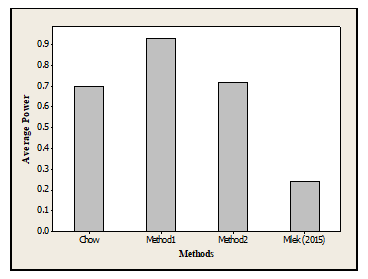Figure 3: Performance of the methods across  the Gamma and Standard Normal Distribution

Also, Method1 was found to perform better than the other methods across the distributions (see table 5). The performance of the methods were in the following order of magnitude Method1=1, Method 2=2, Chow=3 and Milek = 4.

4.4.  Real Life Application of the Methods

Example 1: Real Life Application of the Methods  for Small Sample Situation

Secondary data collected from the National Bureau of Statistics and Central Bank of Nigeria (CBN) statistical bulletin  on Real GDP and Electricity net generation in Nigeria from 1989–2015 was used to illustrate the methods (see Table 1). This example was considered as small sample case since the data points/number of observation were 27. The methods were used to test whether the introduction of Nigeria Electricity Regulatory Commission (NERC) in the year 2005 has significant impact on economic growth in Nigeria. This implies testing for structural break at year 2005. The method 1, 2 and Milek (2015) permutation methods were performed for 10, 000 permutation. The result obtained was summarized in table 6.

Table 6: Performance of the Methods  for example 1

Methods	Chow	Method1 (Ref= 849.087)	Method2 (Ref= 849.087)	Milek (2015) (Ref= 409.81)
P-value	0.000	0.005	0.005	0.005

The result of the example 1, real life application presented in table 6 found a Chow test value of 849.087 which was used as the reference value for the proposed permutation methods for Chow test. The result revealed p-values of 0.005, 0.005, and 0.005 for Method 1, Method 2 and Milek respectively. This result implies that all the methods were able to detect the presence of structural break at break point 2005.

Example 2: Real Life Application of the Methods for Large Sample Situation

This example employed secondary data collected from the records of patients at Federal Hospital Kaura-Namoda, Zamfara State. The data comprises of monthly reported cases of appendicitis from 2011 to 2017. This example was considered as large sample case since the data points/number of observation were above 30. The methods were used to test whether there exist structural break at point 49. This implies testing for structural break at January, 2015 when the President Buhari administration  started (t_a=49). The method 1, 2 and Milek permutation methods were performed for 10, 000 permutation. The result obtained was summarized in table 7.

Table 7: Performance of the Methods for example 2

Methods	Chow	Method1 (Ref= 526.79)	Method2 (Ref= 526.79)	Milek (2015) (Ref= 486.94)
P-value	0.000	0.0049	0.0196	0.0194

The result of the example 2, real life application presented in table 7 found a Chow test value of 526.79 which was used as the reference value for the proposed permutation methods for Chow test analysis. The result revealed p-values of 0.0049, 0.196, and 0.0194 for Method 1, Method 2 and Milek respectively. This result implies that all the methods were able to detect the presence of structural break at break point 49.

5. Conclusion

      This study proposed two new permutation methods for Chow test analysis. The study compared the performance of the proposed permutation methods against the traditional Chow test method and the Milek permutation for structural break using the gamma distribution and the standard normal distribution. Method1 was found to perform better than Method2 followed by the traditional Chow test analysis for both the gamma and standard normal distribution. While the Chow test analysis was found to perform better than the Milek permutation for structural break.

      The result of the example 1, revealed that all the methods were able to detect presence of structural break at break point 2005. Hence, we conclude that the introduction of NERC in 2005 has significant effect on economic growth in Nigeria with regards to electricity net generation. Similarly, the result of the example 2, revealed that all the methods were able to detect presence of structural break at break point 2015. This indicate that the emergence of the president Buhari administration has significant impact on the number of reported cases of appendicitis at Federal Hospital Kaura-Namoda, Zamfara State, Nigeria.

      In view of the outcome of the study, it is recommended Method1 (permute the dependent variable of the full model) be used for detecting structural break in linear models until future studies proves it otherwise.

Conflict of Interest

The authors declare no conflict of interest in this study.

Acknowledgment

We appreciate review comments and inputs from Prof. O. I. Chiaghanam, Prof. S. I. Iwueze, Prof. C. F. R. Odumodu, Dr. Osuji, G. A., Dr. Umedum, C. U. and Dr. G. U. Ebuh in making this work a success.

1.  B. Chen, Hong, Y. “Testing For Smooth Structural Changes In Time Series Models Via Nonparametric Regression” Econometrica, 80(3), 1157–1183, 2012. https://www.jstor.org/stable/41493847. DOI:10.3982/ECTA7990
2.  J. Wongsosaputro, L. L. Pauwels, and F. Chan “Testing for structural breaks in discrete choice models” 19th International Congress on Modelling and Simulation, Perth, Australia, 12–16 December 2011.
3. P. Schmidt and R. Sickles “Some Further Evidence on the Use of the Chow Test under Heteroskedasticity” Econometrica, 45(5), 1293-1298, 1977. DOI: 10.2307/1914076
4.  E. S. Edgington “Randomization Test”. Marcel Dekker, New York. DOI: https://doi.org/10.1007/978-3-642-04898-2_56
5.  B. F. J. Manly “Randomization, Bootstrap and Monte Carlo Methods in Biology, 3rd edition” Chapman and Hall, London, 2007.
6.  D. A. Jackson and K. M. Somers “Are probability estimates from the permutation model of mantel’s test stable?” Canadian Journal of Zoology, 67(3): 766–769, 1989.
7.  C. O. Aronu, G. U. Ebuh “Application of mantels permutation technique on asphalt production in Nigeria. International Journal of Statistics and Applications”, 3(3): 81–85, 2013.
8.  B. Phipson, G. K. Smyth “Permutation p-values should never be zero: calculating exact p-values when permutations are randomly drawn” Statistical Applications in Genetics and Molecular Biology, 9(1), Article 39, 1-12, 2010.
9.  B. S. Cade “Linear Models: Permutation Methods”. Encyclopedia of Statistics in Behavioral Science, 2: 1049-1054, 2005.
10.  M. Ojala, G. C. Garriga “Permutation Tests for Studying Classifier Performance”. Journal of Machine Learning Research, 11: 1833-1863, 2010.
11.  A. M. Winkler, G. R. Ridgway, M. A. Webster, S. M. Smith, T. E. Nichols “Permutation Inference for the general Linear Model” Neuroimage, 92, 381-397, 2014.
12.  Z. Achim, T. Hothorn “A Toolbox of Permutation Tests for Structural Change” Springer-Verlag Statistical Papers, 54(4), 931–954, 2013. https://link.springer.com. doi:10.1007/s00362-013-0503-4
13.  H. Strasser, C. Weber “On the Asymptotic Theory of Permutation Statistics”. Mathematical Methods of Statistics, 8, 220–250, 1999.
14.  M. Milek “Detecting structural changes in the time series in the use of simulation methods” The 9th Professor Aleksander Zelias International Conference on Modelling and Forecasting of Socio-Economic Phenomena, Cracow University of Economics and the Committee on Statistics and Econometrics of the Polish Academy of Sciences, Zakopane, Poland. Pp:145-153, 2015.
15.  G. C. Chow “Tests of Equality between Sets of Coefficients in Two Linear Regressions” Econometrica, 28.3: 591–605, 1960.
16.  A. M. Mood “Introduction to the theory of statistics” New York, NY: McGraw Hill, 1950.
17.  T. E. Davis “The consumption function as a tool for prediction”, Review of Economics and Statistics, 6(34), 270-277, 1952.
18. P. Legendre “Comparison of Permutation Methods for the Partial Correlation and Partial Mantel Tests. J. Statist. Comput. Simulation, (67), 37 – 73, 2000.

(Click Here)

(Click Here)