1. Introduction

Vehicle routing problem (VRP) consists in determining a set of routes to visit a fixed set of customers, in order to minimize the total path length. Several versions of the VRP exist. If each customer specifies availability time windows, we deal with a VRP with Time Windows (VRPTW). Basic variants of the VRP consider the route planning for a vehicle fleet in a single period (shift). In this case, vehicles should come back to the depot before the shift ends. This problem is derived from a healthcare routing question. The healthcare company regularly dispatch products to medical sites. In this case, if overtime is allowed, performance could be significantly upgraded [1]– [4]. For instance, if a location scheduled in the next shift is on the current return path to the depot, a limited overtime allows vehicle serving it. This can significantly diminish next shift workload.

Investigation on the connection between health status and work hours documented concern about the influence of working long hours on people fitness [5]. Furthermore, working long hours increases the chance of micro-sleep in car drivers [6]. In these conditions, the company could be accused of vehicle collision due to enormous workload planning [7]. In fact, shift scheduling objective should limit both anxiety and harmful consequences on healthiness maintaining the work shift as steady as possible.

In an effort of limiting extra time, uncertainty effect on scheduling has to be restricted. Frequently, in optimization problems, data are supposed to be known with certainty. Nevertheless, in practice this is rare. Most commonly, the real data depend on uncertainty because of their irregular essence. Because the optimization problem solution usually reveals a great inclination to the data disturbances, neglecting the data ambiguity may conduct to suboptimal or infeasible solutions for a real case. Stochastic VRP (SVRP) was introduced in [8]. See [9] and [10] for a complete review of SVRP.

Robust optimization is a significant technique to deal with optimization problems subject to uncertainty [11]. The main motive for considering robust optimization is the non-stochastic nature of uncertain parameters. In such a case, a methodology is required to analyze compromise between performance and robustness.

Fuzzy set theory is a useful approach to handle uncertain information, while the stochastic approach is suitable to manage the stochastic parameters in VRP [12]. Some VRP papers utilize fuzzy sets theory for studying the influence of uncertain factors [13]–[23].

In this work, the VRP in a fuzzy random context is analyzed and the fuzzy random theory is adopted to manage such uncertain data. Fuzzy random variables illustrate a well-formalized notion involving data obtained from a random test in which data are supposed to be fuzzy sets.

We examine a multi-shift VRP with no overtime allowed considering fuzzy driving and job processing time. The question we considered is derived from a routing problem in maintenance activities. A maintenance team performs jobs in different sites using a vehicle for movements. A crew works in shifts and should come back to the depot before the shift ends. The goal is completing the maintenance activities in various places reducing the makespan. Since we deal with maintenance jobs, we ignore customer waiting times. We investigate the influence of the uncertainty of driving and job processing time on makespan and overtime avoidance.

The body of this paper is structured as follows. In Section 2, we report the problem formulation. In Section 3, we propose the Artificial Immune Heuristic to solve the problem. We present in Section 4 a case study analyzed with the proposed approach. We give concluding remarks in Section 5.

2. Problem formulation

2.1. Classical problem

Problem notation is reported in Table 1.

Let N = {1,2,…,n} be the set of maintenance jobs to be executed at customer places. Parameter d_i,j stands for the travel time between the location of jobs i and j. Parameter q_i expresses job i processing time. Parameters e_i and l_i represent job i time window.

Maximum shift duration is L, whereas p is the number of shifts in the scheduling horizon and P = {1,2,…,p} is shift set. We generate p + 1 depot copies described by nodes n+1,…,n+p +1:

• node n+1 is the origin depot of shift 1,
• node n + h represents the destination depot of shift h − 1 together with the origin depot of shift h, with h ∈ 2,…,p.
• node n+p +1 stands for the destination depot of last shift p.

The problem can be represented as a directed graph

G = (V ,E), where V = N ∪ {n + 1,…,n + p + 1}. Arcs

(n+h,n+h+1) are used in the graph to illustrate cases in which a vehicle is not exploited during shift h.

Lastly, b_h and c_h represent the begin and end time of shift h, with b_h = (h − 1)L and c_h = hL, h ∈ P .

In this work, the next hypotheses are made. Driving times are positive, i.e. d_ij > 0,∀i,j ∈ V . The triangular inequality is valid for d_ij , i.e. d_ij ≤ d_ik +d_k,j,∀i,j,k ∈ V . At least any single job can be executed in a shift because we suppose shift length satisfies L ≥ d_0,i + q_i + d_i,n+1,∀i ∈ N. Time windows are greater than the activity processing time: l_i − e_i ≥ q_i, ∀i ∈ N. Consequently, a linear formulation for VRPTW is considered. Moreover, a feasible distance set is defined and all the jobs can be processed within their time window and shift duration.

In the following, decision variables are presented:

• x_i,j = 1 if the crew drives from node i to j, and 0 otherwise,
• α_i arrival time of the crew at node i ∈ V ,i , n+1,
• δ_i departing time of the crew at node i ∈ V ,i , n+p +1,
• σ_h real shift h duration,
• y_h = 1 if shift h is used by the crew, and 0 otherwise,

The problem is expressed as a mixed integer program (MIP) described in (1)-(13):

• The objective function (1) minimizes the system makespan.
• Constraints (2) and (3) provide that the depot nodes {n+1,…,n+p +1} are always visited. Depot node n + h + 1 is visited after n + h. Depot nodes separate different shifts. All job nodes visited between node n+h and n+h+1 are served during shift h. If the vehicle is not used in shift h, no job node is visited between node n+h and n + h + 1. Such constraints assure that any shift path starts from the origin depot and ends at the destination depot.
• Constraints (4) ensure that each customer is visited once, that is each node i ∈ N is inspected once.
• Constraints (5) force that for all intermediate nodes (first node n+1 and last node n+p +1 are excluded) the inflow is equal to the outflow.
• Constraints (6) are the sub-tour elimination constraints and ensure coherence of time variables. Parameter M is an upper bound of δ_i +d_ij,∀i,j ∈ V .
• Constraints (7) represent the connection between arrival and departing times.
• Constraints (8)-(9) define time window constraints for the customer nodes, whilst (10)-(11) represent the time windows constraints for the depot nodes.
• Constraints (12) provide the real shift duration. Considering (10)-(12), parameter L is an upper bound of shift duration σ_h, ∀h = 1,…,p.
• Constraints (13) determine whether shift h is exploited or not. In fact, if x_n+h,n+h+1 = 1, then no demand node is inspected between depot h and h+1 (shift h).

Symbol Description n Number of Jobs N = {1,2,…,n} Job set i,j ∈ N Job index di,j Travel time between job i and job j locations qi Job i processing time ei Begin of job i time window li End of job i time window L Maximum shift duration p Number of shifts in the planning horizon P = {1,2,…,p} Shift set h ∈ P Shift set index bh Begin time of shift h, equals to (h − 1)L ch End time of shift h, equals to hL xi,j ∈ {0,1} Crew travels from node i to j, if xi,j = 1 δi Departing time of crew at node i ∈ V ,i , n+p +1 αi Arrival time of crew at node i ∈ V ,i , n+1 σh Actual shift h duration yh ∈ {0,1} Crew is active in shift h, if yh = 1 M Upper bound of δi +dij,∀i,j ∈ V . 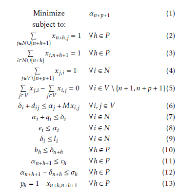Table 1: Problem notation

2.2         Problem with fuzzy uncertainty

We describe the uncertainty on driving times and job processing times with triangular fuzzy numbers, see Fig. 1. We consider the following notation:

• fuzzy travel time: deij = (d_ij^A,d_ij^B,d_ij^C) ∀i,j ∈ V
• fuzzy job processing time: _eq_i = (q_i^A,q_i^B,q_i^C) ∀i ∈ N

For this reason, decision variables related to arrival and departing time at node i turn into fuzzy variables α_ei and δ_ei. Also, actual shift duration variables σ_ei become fuzzy. Therefore, fuzzy numbers are introduced both in objective function (1) and constraints (6)-(12).

An important issue arises when models with fuzzy parameters are considered: defining the comparison method for objective function values [24]. In order to solve this question, we have to consider the ranking of fuzzy numbers [25, 26, 27]. The fuzzy ranking method is part of the solution approach in order to solve mathematical programs having coefficients of the objective function and coefficients of the constraints represented by fuzzy numbers.

The Expected Existence Measure (EEM) operator can be applied to a temporal fuzzy number_et, see (14) and [28, 29].

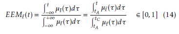Briefly, EEM defines the possibility with which a fuzzy event occurred at a certain time. Assigned a temporal value t₀, the EEM stands for the possibility a temporal fuzzy number _et is lower than t₀. We denote this as Φ(_et ≤ t₀) = ^EEM_et(t₀) = γ₀. Consequently, Φ(_et ≥ t₀) = 1 − γ₀. In Fig. 1, the membership function µ_et(t) of the triangular fuzzy number t˜ and the corresponding EEM_et(t) are represented. Note that Φ(_et ≤ t^A) = EEM_et(t^A) = 0 and Φ(_et ≤ t^C) = EEM_et(t^C) = 1.

Various studies solve fuzzy mathematical problems by exploiting fuzzy ranking methods. First, fuzzy mathematical programming problems are converted into classical mathematical problems. Second, conventional techniques are applied. In the following section, we propose an innovative approach to consider the fuzzy variables in the entire solution process. We present the decision-maker with different optimal solutions based on 2-factor comparison: the objective function value and the possibility degree with which constraints are satisfied.

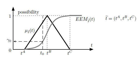Figure 1: Triangular Fuzzy Number

In the previous work [30] we published on this question, we dealt with a different objective function: number of exploited shifts and maximum shift duration. In this research, we consider a different problem in which makespan is minimized. Furthermore, the solution algorithm has been improved with an appropriate solution ‘affinity’ definition in Section 3.2. Moreover, we extended the experimental campaign in order to investigate our approach performance. For such a reason a mathematical background is introduced in sections 4.2, 4.2.2, and 4.2.3.

3. Solution Method: Artificial Immune Heuristic

The animal immune system is a versatile pattern recognition system that protects against foreign viruses and bacteria. The immune system is able to recognize and kill germs. The immune system cells, named antibodies, are casually diffused in the body. The system reacts to pathogens and improves the process of recognizing and eliminating pathogens by using two principles: clonal selection and affinity maturation. When a pathogen invades the organism, clonal selection creates a number of immune cells that recognize and eliminate the pathogen. While cellular reproduction occurs, the cells experience high rate physical mutations, as well as a selective process. Cells with superior affinity to the invading pathogen spread into memory cells.

Artificial Immune Algorithm (AIA) is a metaheuristic based on such system [31, 32, 33]. This paper intends proposing a fuzzy artificial immune algorithm to find optimal solutions for the aforementioned problem. AIA notation is reported in Table 2.

3.1. Solution Encoding

A solution is encoded as a string by using a fixed-length integer code and providing the order in which nodes are reached. Solution Ψ , representing a scheduling problem with n = 5 jobs on p = 3 available shifts, is reported in Fig. 2. Moreover, Fig. 2 shows the corresponding graph path, see section 2. The origin for shift 1 is node n+1 = 6 that is the path starting node. Then, the crew visits nodes 2, 3 and 5. Shift 1 ends at node n+2 = 7. After, shift 2 begins and crew inspects nodes 1 and 4. Shift 2 ends when node n + 3 = 8 is reached. Finally, node n+p+1 = 9 is reached (path end) because no job is executed in shift 3.

Because node (n+1) and (n+p +1) are respectively the ‘starting’ and ‘end’ node, solution Ψ is just defined by the succession of the residual nodes of the graph, that is v_{`</sub> ∈ V \{n+1,n+p+1}, ∀` = 1,…,n+p−1. Note that when x_ij = 1, i,j ∈ V ,i , n + 1,j , n + p + 1, then nodes i and j are directly connected in the graph, consequently ∃` = 1,…,n+p − 2: v<sub>`} = i and v<sub>`+1</sub> = j, that is nodes i and j are consecutive in the string encoding. In Fig. 2 we have x<sub>14</sub> = 1, consequently ∃` = 5, v₅ = 1 and v₆ = 4.

Considering fuzzy numbers, we have to appropriately evaluate both the solution objective function f and solution feasibility degree γ.

First, considering the solution Ψ and adopting the fuzzy addition operator described in (15), we calculate actual duration of shift 1, σ_e1, and shift 2, σ_e2, see (16)(17). Because shift 3 is not used by the crew, we have the same arrival time at node 8 and 9: α_f9 = α_f8. We calculate fuzzy makespan as α_f9 = α_f8 = L+σ_e2. Indeed, makespan is the crew arrival time at the depot at the end of shift 2 (node 8), that is the sum of shift 2 begin time L and actual shift 2 duration σ_e2. Since σ_e2 is a fuzzy number, the crisp objective function f in (18) can be adopted using the modal value σ₂^B of the fuzzy number σ_e2.

Symbol Description popsize No. population antibodies ng No. generations pr1 Rate of Rule1: full random node selection pr2 Rate of Rule2: higher probability for closer node selection, pr2 = 1 − pr1 nc No. clones in each generation mr Mutation Rate nm No. mutations in each generation nea No. exchangeable antibodies. Ψ Solution v` Solution encoding, ∀` = 1,…,n+p − 1, v` ∈ V \ {n+1,n+p +1} f Solution makespan γ Solution feasibility degree S Solution set, |S| = popsize Γ solution Pareto set, Γ ⊂ S AS(f ,γ) Affinity for solution (f ,γ) in set S exp No. experiments in the campaign E experiment set, E = {1,…,exp} Experiment index,  ∈ E E Γ Hyper Pareto set: dominant solutions for set S∈E Γ ρ Impact of experiment Table 2: AIA notation

Second, we determine the degree with which the solution Ψ is feasible. So we calculate the possibility the shift duration constraints are enforced: Φ(σ_e1 ≤ L) = γ₁ and Φ(σ_e2 ≤ L) = γ₂. Time windows constraints are considered in the same way. Supposing for solution Ψ , fuzzy shift durations σ_e1 and σ_e2 are those reported in Fig. 3, it is possible that shift 1 actual duration is greater than maximum limit L. Indeed, half of fuzzy number σ_e1 stays on the right side of L. The value γ₁ = EEM_σe1(L) = 0.5 < 1 indicates the possibility that shift 1 ends before time L. Since, γ₂ = EEM_σe2(L) = 1, shift 2 duration constraint is certainly enforced. Finally, the solution Ψ feasibility degree γ in (19) is determined γ = 0.5.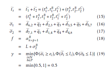

Eventually, for a given solution, we associate a crisp objective function value f and a feasibility degree γ. We perform a Pareto comparison on (f ,γ) pairs for determining the solution Pareto set Γ: f should be minimized and γ should be maximized.

For example, we consider an alternative solution

Ψ in which all the available 3 shifts are exploited. The

0 alternative solution Ψ is reported in Fig. 4. Unlike the

0 previous solution Ψ , in Ψ Job 5 has moved from shift 1 to shift 3. On one hand, we have objective function f = 2L+σ₃^0B, see (18). On the other, for Ψ ⁰ , we have γ is equal to 1 because all shift duration constraints are definitely enforced (γ_i = 1, ∀i = 1,…,N), see σ_h^C <0 1,

∀h = 1,2,3 in Fig. 4. Comparing the solution Ψ to the previous one Ψ , we note that f value gets worse

(f ^Ψ > f ^Ψ ) and γ values is better (γ^Ψ > γ^Ψ ). Indeed, with the alternative solution, shifts are completed in time but one additional shift is required. Since we adopt a 2-factor comparison, both solution Ψ and so

3.2. Affinity

Usually, in meta-heuristic approaches as AIA, an affinity level to be maximized is defined in order to take into account both solution objective value and constraint enforcement. Unfeasible solutions are penalized in terms of affinity. Solutions are ranked on the basis of their affinity values and, eventually, the one with the greatest affinity is defined as ‘best solution’. In our approaches, two different factors (f and γ) are both considered in determining the affinity. Solutions having γ = 0 are certainly unfeasible.

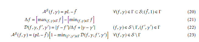
We define the solution set as S. Solutions in the Pareto set Γ = {(f ,γ)|γ > 0} ⊂ S represent the optimal set, and we assign them the same maximum affinity value as in (20). Note that f¯ is the makespan of the solution having feasibility degree 1. Since f stands for makespan to be minimized, whereas affinity is to be maximized, we put f¯ in the second term as the makespan upper bound pL occupies the first term.

Using the normalized Manhattan distance from Pareto set (22), the affinity for solutions not in the Pareto set is computed (23). That is, considering a solution (f ,γ) not in Γ, the minimum Manhattan distance from Pareto set is calculated and is used as a penalty for affinity. Quantity ∆f is used as a weight in Manhattan distance for balancing the effects of makespan and feasibility degree.

3.3         Artificial Immune Algorithm

The proposed AIA is described in the following: Step 1 – Initialization:

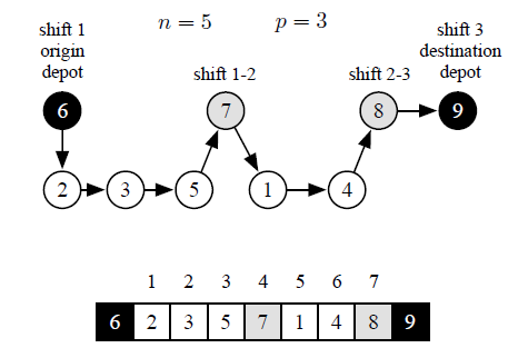Figure 2: Solution Ψ graph path and encoding

• (a) Parameter setting: fix the initial population popsize, the number of generations ng, the rate pr1 of Rule1, the rate pr2 of Rule2, for each generation the number of clones nc, the mutation rate mr, the number of mutations nm, the number of exchangeable antibodies nea.
• (b) Initial population generation: create pr1 · popsize initial solutions by Rule1 and produce pr2 · popsize initial solutions by Rule2.

Step 2 – Objective function assessment:

• (a) calculate the objective function f in (18) and the feasibility degree γ in (19) for each antibody. • (b) determine the Pareto set for (f ,γ) pairs.
• (c) calculate the affinity for each antibody as reported in (20) and (23).

Step 3 – Clonal selection and expansion:

• (a) Take nc antibodies, from the population, with the greatest affinity.
• (b) Produce nc copies of the antibodies considered in Step 3a exploiting a binary tournament rule (randomly select two antibodies from nc antibodies and determine the best antibody).

Step 4 – Generating the next population:

• (a) Randomly choose nm antibodies from nc clones and use the mutations to create nm extra antibodies. Apply each mutation operator with the probability mr.
• (b) Include the nm extra antibodies to the current generation.
• (c) Exchange nea worst antibodies with new ones produced like those in Step 1b.
• (d) Copy the Pareto optimal antibodies to the next generation.

Step 5 – Conclusion test:

• (a) If the stopping criterion is met, return the

Pareto optimal antibodies; otherwise, go to Step 2

At Step 1a, Rule1 is the full random rule: we randomly select one by one the nodes in the set V \ {n +1,n + p +1}. While in Rule2 we choose nodes using a probability that is inversely proportional to the distance between the current node and candidate node. Mutation operator randomly selects two solution indexes (Section 3.1) and swaps content. If the mutation makes unfeasible the depot node sequence n+2,…,n+p, mutation is canceled.

Considering the ordinary AIA approach, the innovation in the method presented in this paper differs in the steps 2b, 2c and 4d. Indeed, step 2b and 2c are used to determine the new antibody affinity. Whereas, step 4d preserves the entire Pareto set in the next generation.

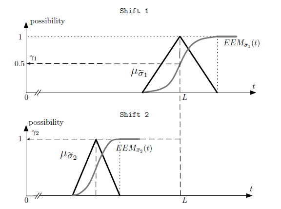Figure 3: Fuzzy shift durations for solution Ψ

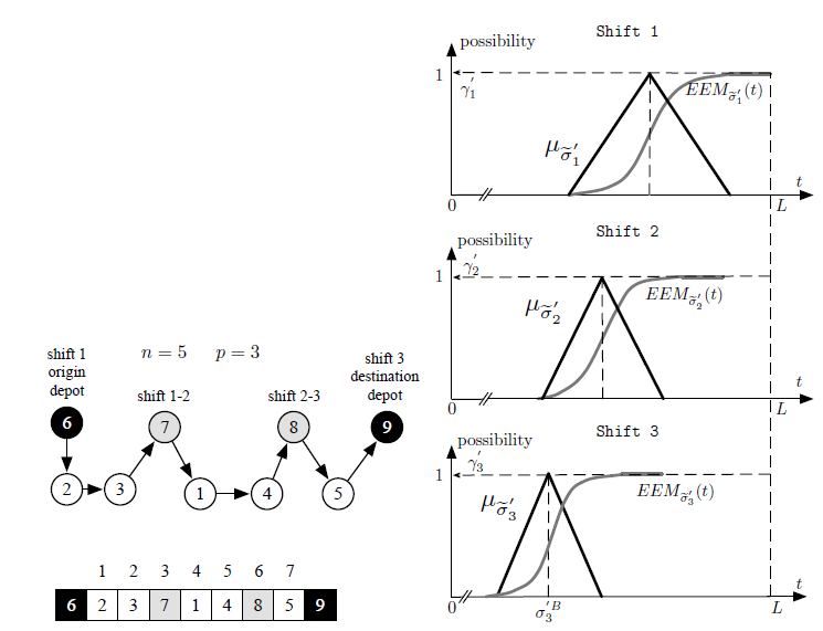Figure 4: Solution Ψ graph path, encoding and fuzzy shift durations

4. Numerical results

We assessed the performance of the approach described in Section 3.3 by generating different experiments. First, considering a standard non-fuzzy problem, we confronted the performance of the MIP reported in (1)-(13) in Section 2, with the AIA, that is Section 3.3 without steps 2b, 2c, and 4d. Second, introducing fuzzy uncertainty, we adopted the AIA reported in Section 3.3 considering innovative steps 2b, 2c, and 4d.

We developed an application on an x86 family 2.5 GHz Intel Core i7 processor having 4GB RAM and SDD, exploiting “C#.Net4” language. In the following, the AIA parameters and their criteria are defined. Population size pop = 200, number of generations ng = 10000, rate for Rule1 and Rule2 pr1 = pr2 = 0.5, number of clones nc = 20, mutation rate mr = 0.75, mutation number per generation nm = 40, exchangeable antibodies number nea = 20.

Three industrial test cases A, B, and C are adopted. In Table 3 the number of demand nodes n and the number of available shifts p is reported. Maximum shift duration is set to L = 480 min. Since industrial records are protected by a non-disclosure agreement, we report only summary data. The considered geographical is the Salento region in southeast Italy. Traveling and processing times are subject to uncertainty and are set considering user-experience values. Job processing times are equally distributed in three groups: small (around 15 min), medium (around 30 min) and large (around 40 min).

4.1.  Non-fuzzy version results

Focusing on the non-fuzzy version of case studies A, B, and C, we compared theperformance of the MIP model in (1)-(13) with AIA. Crisp values t^B are considered in place of the fuzzy version t˜. The non-fuzzy MIP model reported in (1)-(13) was solved with software package IBM CPLEX v.12.5 setting a time limit equal to the running time of the AIA application. In Table 4 we described the achieved results. In particular, for each case study and for each approach, we indicated the time (sec) when a new better solution is detected together with the corresponding solution optimal gap (%). In the first case study A, AIA calculates formerly the MIP optimal solution. For case study B, the optimal solution gap of AIA from MIP is 1% but AIA is tenfold faster than MIP. Finally, in the case study C, the optimal gap is 4%.

4.2. Fuzzy version results

Considering the fuzzy version of case studies A, B, and C, we adopted the fuzzy AIA to obtain the solution Pareto set. As reported in Section 3, multiple optimal solutions exist because of the 2-factor comparison. Company manager receives the optimal Pareto set and assesses the best solution. In Section 4.2.1, an example is provided. Assuming different AIA parameter values leads to different Pareto sets as shown in Section 4.2.2.

Our main objective consists in determining the AIA parameters to find as many Pareto set solutions. Consequently, we designed an experimental campaign to determine the best combination of AIA parameter values, see Section 4.2.3. Each experiment  produces a solution Pareto set Γ. Considering all the campaign experiments E = {1,…,exp} leads merging the corresponding Pareto sets ^S∈E Γ. Union of Pareto sets is not a Pareto set, because a solution of a Pareto set can be dominated by a solution of another Pareto set experiment. We define Γ as Hyper Pareto set for experiments 1,…,exp containing only the dominant solutions obtained from the experimental campaign. For each experiment , we denote the experiment impact ρ as the number of solutions belonging both to the experiment Pareto set

Table 3: Case study definition

Case study	n	p
A	21	5
B	33	8
C	45	10

4.2.1        Single experiment results

Considering the fuzzy version of case study A, our software produces the Pareto set reported in Fig. 5. The collected solutions s1,s2,…s10, belonging to the optimal Pareto set, are reported in Table 5. For such solutions, jobs are always completed in 3 shifts.

Feasibility degree for solution s1 is 1, because σ_i^C < 480, ∀i = 1,2,3. Solution s1 makespan is 2·480+348 = 1308 min. Since solution s1 is very conservative, the manager is unlikely to accept such a high safety margin.

Whereas, solution s2 has f = 1263 min and γ = 0.968. Indeed, in Table 5 we have σ₁^C = 486 > 480 and σ₂^C = 499 > 480; we note that 96.8% of the area of fuzzy number σ_e2 = (349;424;499) stays on the left side of 480 (see Fig. 1). The manager prefers solution s2 to s1 as assuming a low risk (3.2%) he/she decreases makespan by 45 minutes. Solutions s3 and s4 have similar feasibility degrees but s4 makespan is lower than s3. Whereas, solutions s5, s6, and s7 have similar makespan but s5 feasibility degree is better than others. Feasibility degrees for solutions s8, s9, and s10 are lower than 0.5: see σ₂^B > 480 min in last three rows in Table 5.

Referring to Fig. 5, manager declares that solutions s2, s4, and s5 are the most valuable and selects the best one based on his/her experience.

In Fig. 6, shift tours for solution s1 are graphically reported using ‘Google Maps’ website (maps.google.com). For privacy agreement, only the position of Lecce, Salento main city, is indicated. Depot position is red pinned. Job locations are indicated with circles. Basically, shift 1 tour accomplishes jobs in the north side. Shift 2 serves central zone and shift 3 satisfies south side. Each shift serves 7 jobs.

Table 4: Comparison AIA vs. MIP for non-fuzzy version of case studies A, B, C

Case study A				Case study B				Case study C
AIA		MIP		AIA		MIP		AIA		MIP
t [sec]	gap [%]	t [sec]	gap [%]	t [sec]	gap [%]	t [sec]	gap [%]	t [sec]	gap [%]	t [sec]	gap [%]
1	130	1	230	1	123	1	450	1	187	1	345
20	95	31	99	31	115	30	129	21	125	36	234
45	43	76	87	51	33	45	97	48	49	54	221
105	22	273	54	120	12	150	65	532	4	169	198
123	0	778	23	246	1	264	51			254	187
		1002	13			778	42			675	85
		1324	6			1042	21			1201	31
		1457	0			1256	14			1312	20
						2001	9			1416	12
						2398	2			2395	7
						2405	0			5998	2
										7194	0

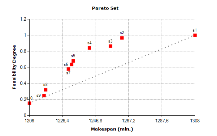Figure 5: Final solution Pareto set for fuzzy case study A with basic parameters

Table 5: Details of final solutions for fuzzy case study A with basic parameters

	Actual Fuzzy Shift Duration σei
Solution	Shift 1	Shift 2	Shift 3
s1	(357;417;477)	(345;410;475)	(298;348;398)
s2	(366;426;486)	(349;424;499)	(263;303;343)
s3	(372;432;492)	(369;444;519)	(256;296;336)
s4	(390;450;510)	(365;445;525)	(248;283;318)
s5	(402;467;532)	(369;444;519)	(238;273;308)
s6	(402;467;532)	(394;469;544)	(237;272;307)
s7	(400;460;520)	(388;473;558)	(240;270;300)
s8	(400;460;520)	(412;497;582)	(226;256;286)
s9	(418;473;528)	(420;505;590)	(220;255;290)
s10	(371;426;481)	(433;518;603)	(211;246;281)

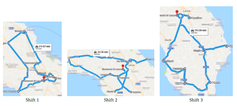Figure 6: Shift tours for the solution s1

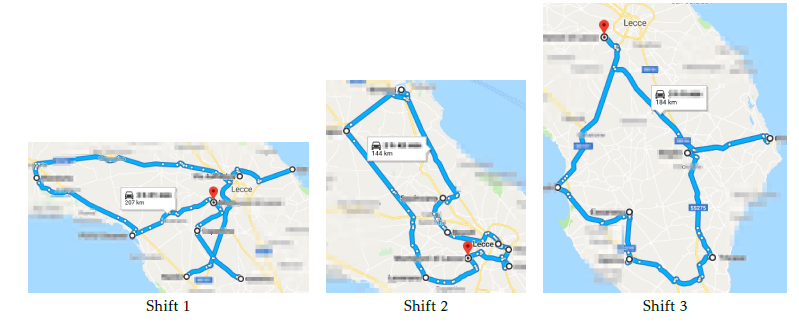Figure 7: Shift tours for the solution s2

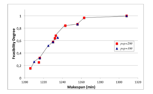Figure 8: Final solution Pareto set for fuzzy case study A with two experiments

Table 6: Experiment impact results

exp	ng	pop	pr1	ρ		exp	ng	pop	pr1	ρ		exp	ng	pop	pr1	ρ
1 2 3	5000 5000 5000	100 100 100	0.25 0.50 0.75	5 5 5		1 2 3	5000 5000 5000	100 100 100	0.25 0.50 0.75	7 7 7		1 2 3	5000 5000 5000	100 100 100	0.25 0.50 0.75	9 9 9
4 5 6	5000 5000 5000	200 200 200	0.25 0.50 0.75	7 8 6		4 5 6	5000 5000 5000	200 200 200	0.25 0.50 0.75	8 11 8		4 5 6	5000 5000 5000	200 200 200	0.25 0.50 0.75	9 14 11
7 8 9	5000 5000 5000	300 300 300	0.25 0.50 0.75	7 8 6		7 8 9	5000 5000 5000	300 300 300	0.25 0.50 0.75	9 11 8		7 8 9	5000 5000 5000	300 300 300	0.25 0.50 0.75	12 15 11
10 11 12	10000 10000 10000	100 100 100	0.25 0.50 0.75	5 6 5		10 11 12	10000 10000 10000	100 100 100	0.25 0.50 0.75	7 7 7		10 11 12	10000 10000 10000	100 100 100	0.25 0.50 0.75	10 9 10
13 14 15	10000 10000 10000	200 200 200	0.25 0.50 0.75	8 9 8		13 14 15	10000 10000 10000	200 200 200	0.25 0.50 0.75	10 12 11		13 14 15	10000 10000 10000	200 200 200	0.25 0.50 0.75	13 16 16
16 17 18	10000 10000 10000	300 300 300	0.25 0.50 0.75	8 9 9		16 17 18	10000 10000 10000	300 300 300	0.25 0.50 0.75	11 12 12		16 17 18	10000 10000 10000	300 300 300	0.25 0.50 0.75	15 16 16
19 20 21	15000 15000 15000	100 100 100	0.25 0.50 0.75	5 6 5		19 20 21	15000 15000 15000	100 100 100	0.25 0.50 0.75	7 8 7		19 20 21	15000 15000 15000	100 100 100	0.25 0.50 0.75	10 11 10
22 23 24	15000 15000 15000	200 200 200	0.25 0.50 0.75	8 9 9		22 23 24	15000 15000 15000	200 200 200	0.25 0.50 0.75	11 13 12		22 23 24	15000 15000 15000	200 200 200	0.25 0.50 0.75	15 18 16
25 26 27	15000 15000 15000	300 300 300	0.25 0.50 0.75	8 9 9		25 26 27	15000 15000 15000	300 300 300	0.25 0.50 0.75	11 13 14		25 26 27	15000 15000 15000	300 300 300	0.25 0.50 0.75	15 18 17

In Fig. 7, tours for solution s2 are reported. The comparison of solution s2 with s1 is described in the following (see Fig. 6 and 7). Shift 1 tour lies in the central area whereas shift 2 concerns the north zone. In s2, to reduce makespan, one job is removed from shift 3 and added to shift 2. A job swap is performed between shift 1 and 2 in order to limit the shift 2 duration.

4.2.2        Two-experiment results

We compare the experiment performed in previous section 4.2.1 ( = 1), with a new experiment ( = 2) in which pop parameter is decreased from 200 to 100. Consequently, considering the experimental campaign set E = {1,2}, we report the corresponding solution Pareto sets Γ₁ (pop = 200) and Γ₂ (pop = 100) in Fig. 8.

Set Γ₁, in red, is reported in Fig. 5 too. Set Γ₂ contains

7 solutions, in particular: 4 solutions belong to Γ₁ too, 2 solutions are dominant solutions not included in Γ₁ and one solution is dominated by another in Γ₁. Instead, one solution in Γ₁ is dominated by a solution in Γ₂. Since, the new experiment ( = 2) produces two additional solutions in Pareto set and removes one, we

have |Γ | = 11. In Fig. 8, the line represents Pareto front. Calculating ρ₁ = 9 and ρ₂ = 6, we can assess that first experiment has a greater impact than second.

4.2.3        Experimental campaign results

Considering the case study described in Section 4, we designed an experimental campaign. We examined 3 parameters ng, pop, and pr1 on 3 different levels: ng ∈ {5000,10000,15000}, pop ∈ {100,200,300}, and pr1 ∈ {0.25,0.50,0.75}. Consequently, for each case study, we have 27 experiments, E = {1,…,27}. For each experiment  ∈ E, we calculate the corresponding impact ρ. In Table 6a, experiment impact values are reported for case study A. As parameter pop increases, we obtain a larger number of Pareto set solutions. Increasing the parameter ng from 5000 to 10000 succeeds in increasing ρ, the same cannot be said when passing from 10000 to 15000. Parameter pr1 has a positive influence when pr1 = 0.50.

In Table 6b and Table 6c, experiment impact values are reported for case study B and C. The results confirm the findings of case study A. In conclusion, our solution Pareto set approach significantly depends on population parameter pop. Indeed, in each generation, we preserve the ‘entire’ solution Pareto set, so it is important having a larger pop value than the non-fuzzy approach. Parameter pr1 = pr2 = 0.50 represents a good compromise between generating Rule1 full random solutions and Rule2 solutions (Section 3.3).

5. Conclusion

This study presents some real insights into the single vehicle routing problem with multi-shift and fuzzy uncertainty. Our objective consists of minimizing both the system makespan and shift overtime occurrence. In particular, we investigated the effect of uncertainty in driving and job processing time. We provide optimal solutions for the decision-maker considering a 2-factor comparison: the objective function value (makespan) and the degree with which overtime is avoided. Our approach is currently used by the case study company.

1.  S. Zangeneh-Khamooshi, Z. B. Zabinsky, and J. A. Heim, “A multi-shift vehicle routing problem with windows and cycle times,” Optimization Letters, vol. 7, no. 6, pp. 1215–1225, aug 2013.
2.  Y. Ren, M. Dessouky, and F. Ord´o˜nez, “The multi-shift vehicle routing problem with overtime,” Computers & Operations Research, vol. 37, no. 11, pp. 1987–1998, 2010.
3.  G. Onder, I. Kara, and T. Derya, “New integer programming formulation for multiple traveling repairmen problem,” Transportation Research Procedia, vol. 22, pp. 355–361, 2017. [Online]. Available: http: //linkinghub.elsevier.com/retrieve/pii/S2352146517301771
4.  S. Nucamendi-Guill´en, I. Mart´inez-Salazar, F. Angel-Bello, and J. M. Moreno-Vega, “A mixed integer formulation and an efficient metaheuristic procedure for the k-Travelling Repairmen Problem,” Journal of the Operational Research Society, vol. 67, no. 8, pp. 1121–1134, aug 2016. [Online]. Available: https: //www.tandfonline.com/doi/full/10.1057/jors.2015.113
5.  K. Sparks, C. L. Cooper, Y. Fried, and A. Shirom, “The Effects of Working Hours on Health: A Meta-Analytic Review,” in From Stress to Wellbeing Volume 1. London: Palgrave Macmillan UK, 2013, pp. 292–314.
6.  C. C. Caruso, “Negative Impacts of Shiftwork and Long Work Hours,” Rehabilitation Nursing, vol. 39, no. 1, pp. 16–25, jan 2014.
7.  G. Costa, “Shift Work and Health: Current Problems and Preventive Actions,” Safety and Health at Work, vol. 1, no. 2, pp. 112–123, 2010.
8.  T. M. Cook and R. A. Russell, “A Simulation and Statistical Analysis of Stochastic Vehicle Routing with Timing Constraints,” Decision Sciences, vol. 9, no. 4, pp. 673–687, oct 1978.
9.  M. Gendreau, G. Laporte, and R. S´eguin, “Stochastic vehicle routing,” European Journal of Operational Research, vol. 88, no. 1, pp. 3–12, jan 1996.
10.  G. Yaohuang, X. Binglei, and G. Qiang, “Overview of Stochastic Vehicle Routing Problems,” Journal of Southwest Jiaotong University, vol. 10, no. 2, pp. 113–121, 2002.
11.  C. Lee, K. Lee, and S. Park, “Robust vehicle routing problem with deadlines and travel time/demand uncertainty,” Journal of the Operational Research Society, vol. 63, no. 9, pp. 1294–1306, sep 2012.
12.  J. Xu, F. Yan, and S. Li, “Vehicle routing optimization with soft time windows in a fuzzy random environment,” Transportation Research Part E: Logistics and Transportation Review, vol. 47, no. 6, pp. 1075–1091, 2011.
13.  H. Ewbank, P.Wanke, and A. Hadi-Vencheh, “An unsupervised fuzzy clustering approach to the capacitated vehicle routing problem,” Neural Computing and Applications, vol. 27, no. 4, pp. 857–867, may 2016.
14.  Z. Zhu, J. Xiao, S. He, Z. Ji, and Y. Sun, “A multi-objective memetic algorithm based on locality-sensitive hashing for oneto- many-to-one dynamic pickup-and-delivery problem,” Information Sciences, vol. 329, no. C, pp. 73–89, feb 2016.
15.  A. G. Novaes, E. T. Bez, P. J. Burin, and D. P. Arag˜ao, “Dynamic milk-run OEM operations in over-congested traffic conditions,” Computers & Industrial Engineering, vol. 88, no. C, pp. 326–340, oct 2015.
16.  H. Zhao, W. A. Xu, and R. Jiang, “The Memetic algorithm for the optimization of urban transit network,” Expert Systems with Applications, vol. 42, no. 7, pp. 3760–3773, may 2015.
17.  D. Mu˜noz-Carpintero, D. S´aez, C. E. Cort´es, and A. N´u˜nez, “A Methodology Based on Evolutionary Algorithms to Solve a Dynamic Pickup and Delivery Problem Under a Hybrid Predictive Control Approach,” Transportation Science, vol. 49, no. 2, pp. 239–253, may 2015.
18.  S. F. Ghannadpour, S. Noori, R. Tavakkoli-Moghaddam, and K. Ghoseiri, “A multi-objective dynamic vehicle routing problem with fuzzy time windows: Model, solution and application,” Applied Soft Computing, vol. 14, pp. 504–527, jan 2014.
19.  D. S´aez, C. E. Cort´es, and A. N´u˜nez, “Hybrid adaptive predictive control for the multi-vehicle dynamic pick-up and delivery problem based on genetic algorithms and fuzzy clustering,” Computers & Operations Research, vol. 35, no. 11, pp. 3412– 3438, nov 2008.
20.  L. de C.T. Gomes and F. J. Von Zuben, “Multiple criteria optimization based on unsupervised learning and fuzzy inference applied to the vehicle routing problem,” Journal of Intelligent & Fuzzy Systems: Applications in Engineering and Technology, vol. 13, no. 2-4, pp. 143–154, 2002.
21.  Y. He and J. Xu, “A class of random fuzzy programming model and its application to vehicle routing problem,” World Journal of Modelling and simulation, 2005.
22.  D. Teodorovi´c and G. Pavkovi´c, “The fuzzy set theory approach to the vehicle routing problem when demand at nodes is uncertain,” Fuzzy Sets and Systems, vol. 82, no. 3, pp. 307–317, sep 1996.
23.  K. Tan and K. Tang, “Vehicle dispatching system based on Taguchi-tuned fuzzy rules,” European Journal of Operational Research, vol. 128, no. 3, pp. 545–557, 2001.
24.  M. Jim´enez, M. Arenas, A. Bilbao, and M. V. Rodrguez, “Linear programming with fuzzy parameters: An interactive method resolution,” European Journal of Operational Research, vol. 177, no. 3, pp. 1599–1609, mar 2007.
25.  H.-J. Zimmermann, M. A. E. Kassem, N. M. El-Badry, and A. Bilbao, “Fuzzy mathematical programming,” Computers & Operations Research, vol. 10, no. 4, pp. 291–298, jan 1983.
26.  M. Jim´enez, “Ranking Fuzzy Numbers Through The Comparison Of Its Expected Intervals,” International Journal of Uncertainty, Fuzziness and Knowledge-Based Systems, vol. 04, no. 04, pp. 379–388, aug 1996.
27.  H. J. J. Kals, International Design Seminar 1999 Enschede, and International Institution for Production Engineering Research, Integration of process knowledge into design support systems : proceedings of the 1999 CIRP International Design Seminar, University of Twente, Enschede, The Netherlands, 24 – 26 March 1999. Kluwer, 1999.
28.  Baoding Liu and Yian-Kui Liu, “Expected value of fuzzy variable and fuzzy expected value models,” IEEE Transactions on Fuzzy Systems, vol. 10, no. 4, pp. 445–450, aug 2002.
29.  Quan Nguyen and Tu Van Le, “Fuzzy discrete-event simulation with FTipLog,” in 1996 Australian New Zealand Conference on Intelligent Information Systems. Proceedings. ANZIIS 96. IEEE, pp. 195–198.
30.  F. Nucci, “The multi-shift single-vehicle routing problem under fuzzy uncertainty,” in 2017 IEEE International Conference on Service Operations and Logistics, and Informatics (SOLI). IEEE, sep 2017, pp. 156–161. [Online]. Available: http://ieeexplore.ieee.org/document/8120987/
31.  M. Mobini, Z. Mobini, and M. Rabbani, “An Artificial Immune Algorithm for the project scheduling problem under resource constraints,” Applied Soft Computing, vol. 11, no. 2, pp. 1975– 1982, mar 2011.
32.  A. Bagheri, M. Zandieh, I. Mahdavi, and M. Yazdani, “An artificial immune algorithm for the flexible job-shop scheduling problem,” Future Generation Computer Systems, vol. 26, no. 4, pp. 533–541, apr 2010.
33.  J. Al-Enezi, M. Abbod, and S. Alsharhan, “Artificial Immune Systems – models, algorithms and applications,” International Journal of Research and Reviews in Applied Sciences, vol. 3, no. 2, pp. 118–131, 2010.

(Click Here)

(Click Here)