1. Introduction

Rapid developments in sensor technology, data processing tools and data storage capability have helped fuel an increased appetite for equipment health monitoring in mechanical systems. As a result, the number of sensors and amount of data collected for health monitoring has grown tremendously. It is hoped that by collecting large quantities of operational data, predictive tools can be developed that will provide operational, maintenance and safety benefits. Data mining and machine learning techniques are important tools in addressing the ensuing challenge of extracting useful results from the data collected. However, incorporating as much physical domain knowledge to the analysis as possible is also necessary to ensure the results are relevant and practical for the operator and end-user.

This work describes continued analysis of sensor data for the turbocharger subsystem of a diesel engine system. The engine has hundreds of sensors monitoring both the inputs of the engine operator and the resulting equipment outputs. A turbocharger seizure was recorded by the diesel engine sensor system. Therefore, data analysis of this incident including the lead up to the event allows for monitoring and identification of changes in equipment condition indicators with a known outcome.

This paper is an extension of work originally presented at the 2017 IEEE International Symposium on Robotics and Intelligent Sensors (IRIS) [1]. The initial data analysis of this event included intrinsic dimension analysis and relied on clustering techniques for data reduction to transform the high-dimensional sensor data to a low-dimensional space. In this extended version of the paper, the data has not been reduced using clustering techniques in order to minimize information loss and t-Distributed Stochastic Neighbour Embedding (t-SNE) is included as an additional mapping method. An important addition in this paper is further analysis to relate individual sensor signals to the internal data structure of the low-dimensional mappings.

Failure detection in mechanical systems using data-driven models is an area that has been the focus of much published research in the last decade or so. Machinery failures are hard to predict due to the complex nature of the structure and functions of the system. Using data driven models helps reduce maintenance costs, improve productivity and increase machine availability [2]. For example, fuzzy support vector machines have been applied to identify faults in induction motors [3]. In another case, various data-driven models such as support vector machines, decision trees and kernel methods were used and compared to diagnose faults in shaft and bearings of rotating machinery [4]. Additionally, a model was developed to continuously monitor the health of wind turbine gearboxes [5]. In brief, data-driven models demonstrate great potential for failure detection and preventive maintenance in mechanical applications.

Other related work revolves around understanding the trends data-driven models produce. In several fields, data is being acquired at an astounding rate [6]. There is a significant need for the development of methods and techniques to obtain useful knowledge from these growing sets of available data. Currently, there exist few processes that combine expert knowledge of a system with algorithm-generated prediction models of the system’s datasets. However, in cases where expert knowledge is combined with machine learning techniques, there is a notable improvement in the results. For example, a methodology was proposed to detect web attacks [7]. In this procedure, features that represented the tendencies of the system were chosen by experts and were combined with output provided by n-grams, a feature extraction algorithm. In another instance, similar to mechanical applications, a framework to combine the clinical intuitions and experience of medical experts with machine learning models was used to overcome the lack of ideal training sets [8]. Medically trained experts provided a task to accomplish, the desired outcome, the data, and helped construct relationships between variables with the algorithm designers. The relationships that were provided aligned with the intuition of the medical expert and their understanding of how factors played out in predicting a certain outcome [8]. However, when expert-knowledge is not always readily available, or if all the variables cannot be identified for a particular outcome, or when proper variable relationships cannot be constructed for a particular outcome, the need to be able to obtain useful knowledge from the results of data-driven models still exists.

In this work, a multi-disciplinary approach to gain knowledge from high-dimensional and voluminous datasets generated by complex real-world systems is explored. Data mining and machine learning techniques are implemented to gather useful insights from the large amounts of sensor data collected for this diesel engine system. By incorporating expert domain knowledge with the low-dimensional representations of the data, a more practical understanding of the data structure presented in the mappings is provided which helps ensure that the results are relevant and accessible to the operator and end-user.

This paper is organized as follows: description of the turbocharger sensor data and the turbocharger seizure are provided in Section 2; details of the implemented data analysis tools and techniques are given in Section 3; the data pre-processing steps and the experimental settings are outlined in Section 4; the intrinsic dimension analysis and low-dimensional mappings are included in Section 5; Section 6 provides the results of several sensor signals overlaid on the visualizations; and finally, Section 7 summarizes the findings of the paper.

2. Turbocharger data

The analyzed turbocharger system contains twin air-cooled turbochargers providing the air-charge to the medium-speed diesel engine system. The diesel engine system consists of two banks of 10-cylinders, denoted Bank A and Bank B. A single turbocharger is assigned to each 10-cylinder bank; the two turbochargers are differentiated as Turbo A and Turbo B, where the letter  ‘A’ or ‘B’ identifies their respective cylinder bank.

The incident recorded by the engines sensor system and analyzed within this work relates to the seizure of Turbo A [1]. The sensor data recorded for this particular incident was available for the month leading up to and including the time of the incident. From the resulting investigation of the Turbo A seizure, a series of key events leading to the incident were noted. The chronology of the incident’s events is detailed below, with the time of occurrence indicated as (hh:mm).

• Noted loss of sensor reading on Turbo A speed sensor
• Engine shut down for inspection
• Turbo A and B speed sensors switched
• Engine restarted at idle, still no Turbo A speed reading indicated (01:12)
• Engaged diesel engine (01:41)
• Higher speed setting requested (01:42), engine exhaust temperatures increased beyond alarm threshold, with no speed increase achieved (01:43 – 01:44)
• Diesel engine disengaged and shut down (01:44 – 01:45)

Following the incident, an inspection of Turbo A was conducted. From the inspection it was determined that the seizure of Turbo A occurred due to a sensor installation error, which occurred when the speed sensors for Turbo A and B were switched. Insufficient spacing between the speed sensor and the turbine’s thrust collar led to rubbing and eventually the turbocharger seizure [1].

Although this failure was caused by installation error rather than gradual deterioration of a system element, the ability to characterize and distinguish the healthy state from the seized state of the turbocharger system using data analysis tools is of significant value. This type of analysis could aid in establishing failure models for further predictive work.

2.1.  Turbocharger sensor signals

The sensor system of the diesel engine is comprised of 238 sensors that capture information related to operator inputs, equipment outputs, and sensor data. The sensor system provides a means for staff to control system components, monitor the systems status, or be notified via alarm when various pieces of equipment operate outside of pre-set threshold values. In addition, the sensor system allows for the recording and archiving of the operational data measured from various instruments at rates up to 2 Hz. From the 238 sensors relevant to the diesel engine, a subset of 31 signals relating to the operation of the turbochargers was selected. The 31 sensors considered within this analysis, listed in Table 1 [1], encompass parameters such as speeds, temperatures (inlet, outlet, and exhaust), pressures, and shaft torque.

The data from the month leading up to and including the turbocharger seizure was analyzed. With the data down-sampled to 1-minute intervals, there were 9968 data points during the time period. The data points prior to the turbocharger seizure were designated as ‘healthy’, while the points from midnight of the date of the incident were considered ‘failed’ points. These failed points include all of the data points after the seizure as they correspond to data related to the seized subsystem. As a result, there were 9875 healthy points and 93 failed points identified.

3. Analytical techniques

An important aspect of this workwas the characterization of the relationship between the healthy and failed states of the turbocharger system, particularly the transition between the two states. The original sensor data is described by a multidimensional time-series composed of the 31 signals. Typical from these kind of data is the presence of noise, irrelevancies and redundancies between the descriptor variables, as in reality the core of the data represents a subspace of lower dimension embedded within the higher dimensional descriptor space. In such situations, transformations to lower dimensional spaces are useful for highlighting and visualizing the underlying structure of the information.

To that end, a suitable transformation, preferably with an intuitive metric [9] would produce a mapping of the original high dimensional objects into a lower dimension one, such that a certain property of the data is preserved by the representation. Desired properties characterizing data structure could be conditional probability distributions around neighbourhoods, similarity relations and others. Under normal circumstances, such transformations imply some information loss or error that should be minimized. If successful, the transformation would generate a new set of features out of the original ones which would preserve the desired property, but in a lower dimension representation space that mitigates the curse of dimensionality.

3.1.  Intrinsic dimensionality analysis

When choosing the dimension of the target space, it is important to consider the intrinsic dimensionality of the original information which is typically understood as the minimum number of variables required to account for the observed properties of the data [10-13]. Given a functional measure of information loss, it is the minimum number of dimensions (descriptor variables) required to describe the data that minimizes that measure. This concept could be understood in several ways, which results in different algorithms aiming at producing such an estimation. Some approaches focus on local properties of the data, whereas other techniques emphasize the analysis of global properties of the data. Most complex systems in the real world exhibit nonlinear relations among their state variables, which make linear estimators of intrinsic dimensionality at a global scale less powerful than their nonlinear estimation counterparts. However, some of them are computationally expensive.

From the practical point of view, the smaller the choice of the target dimension with respect to the intrinsic one, the higher the representation error would be. On the other hand, choosing values higher than the chosen dimension introduce unnecessary attributes, redundancies and possibly noise. For visualization purposes, three or two dimensions are forcibly required. In these cases, the value of the intrinsic dimension provides a useful guide to the level of caution required when making inferences based on the visualization space.

In this work, the intrinsic dimension of the turbocharger data is estimated using four nonlinear methods and one linear technique: maximum likelihood estimation (MLE), correlation dimension (CD), geodesic minimum spanning tree (GMST), nearest neighbour estimator, and principal component analysis (PCA).

The maximum likelihood estimator [14] is based on the assumption of a Poisson distribution for the k neighbour points and a constant behavior of the probability density function around a given point. The actual estimate of the dimension is derived from the log-likelihood function.

Correlation dimension [15] is one type of fractal dimension and it is one of the most commonly used techniques for estimating the intrinsic dimension. The idea is to compare objects from the point of view of their pairwise distances, producing a normalized count of those pairs whose distance does not exceed a given threshold (the correlation integral). The estimate is given by the slope of a log-log linear regression of the correlation integral values vs. the different distance thresholds r.

The geodesic minimum spanning tree (GMST) estimator [16] assumes that i) the set of multivariate objects are in a smooth manifold embedded within the higher dimensional space determined by the original descriptor variables and ii) these objects are realizations of a random process from an unknown multivariate probability density distribution. This technique produces an asymptotically consistent estimate of the manifold dimension without requiring the reconstruction of the manifold or the estimation of the multivariate distribution of the objects. The first step is to construct a graph based on k-neighbourhood density (or neighbourhood distances) where every object is connected with the others nearby. The second step is to build a minimal spanning tree (MST). The distances along its edges and the overall length are used to estimate parameters of the manifold, like entropy and dimension.

The nearest neighbour estimator [17] presents some similarities with the correlation dimension. It is motivated by the possibility of approximating the unknown probability density of the set of multidimensional objects, by normalizing the relative number of nearest neighbours by the volume of the hypersphere containing the objects. The procedure computes the smallest radius r required to cover k nearest neighbours via a linear log-log regression of the average minimum radius vs. k.

Principal component analysis (PCA) is an unsupervised, classical method that is among others, it is used to estimate intrinsic dimensionality. The estimation is simply constructed by obtaining the number of eigenvalues whose relative contributions to the overall variance exceeds a predetermined threshold (e.g. 0.975). Singular value decomposition techniques or diagonalization of covariance/correlation matrices are the typical approaches used for finding the components, which are linear combination of the original set of features. The former approach was used in this paper following the algorithm described in [18].

3.2.  Transformation from high- to low-dimensional space

The specificities of the data determine its intrinsic dimension and, in particular, when the estimates are not too different from three, mappings targeting that number of dimensions could portray appropriate representations of the data. In these cases, the visualizations obtained with different mapping techniques typically exhibit low errors or information loss measures. They would reveal patterns corresponding to valid relationships within the data like regularities, showing up as clustering structure, as well as abnormalities, less frequent elements and outliers.

Clearly, for machine learning purposes, mitigating the curse of dimensionality is important and often the dimension of the target spaces must go beyond the ones required by visual inspection. In this paper, Principal Components, Sammon mapping, t-SNE and Isomap were used as representatives of linear and nonlinear transformation techniques.

Principal Components

A low-dimensional representation of the data can be produced using the first few principal components found through principal component analysis, which are mutually orthogonal (described in Section 3.1). Their main features were presented in the previous section. From the point of view of visually inspecting the data, the first few principal components (up to three) are used as a baseline low-dimensional representation. They are linearly uncorrelated and the amount of variance contained in each new component decreases monotonically. However, the cumulated variance contained in the first three components is not sufficiently high and it is a crucial element to consider when working with principal components visualizations.

Sammon Mapping

The idea of constructing low dimensional spaces where the distance distribution maximally matches the one in the original space is very intuitive and has been at the core of multi-dimensional scaling methods (MDS) [19-22]. Different variants of this approach have been used for creating visual representations of metric and non-metric data. On representations that aim at preserving distances in the original and the target spaces, nearby/distant objects in the original data space are placed at nearby/distant locations from each other in the low-dimensional target space. Some variants preserve the actual distance values, while others aim at preserving their ranks or their ordering relation.

In the first case, measures based on squared differences between dissimilarities on both spaces are commonplace and are variations of objective functions like

where N is the number of objects, w_ij is a weight associated to every pair of objects i, j, F is a monotonically increasing function, δ_ij is a dissimilarity measure between objects i, j in the original data space and d_ij is their dissimilarity/distance in the target space, with p as an exponent of the difference term.

From this general formulation, several mapping techniques are derived, in particular, Sammon’s nonlinear mapping [23], conceived as a transformation of vectors of two spaces of different dimension (D >m) by means of a function , which maps vectors  to vectors , . The actual objective function to minimize is given by Equation 1:

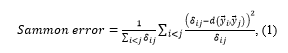where typically d is an Euclidean distance in . The weight term  highlights the importance of smaller distances and therefore, the behavior around close neighbourhoods exerts a larger influence on the error function.

t-SNE

A probabilistic principle is used by the Stochastic Neighbour Embedding (SNE) [24], where the goal is to preserve neighbour identities. A dissimilarity or distance between the objects in the original space is used for creating an asymmetric probability for each object with respect to its potential neighbours, with a pre-set neighbourhood notion (the perplexity). The same is performed for the objects in the target space.

The goal is to match the two distributions as much as possible, which is achieved by minimizing the sum of Kullback-Leibler divergences. The rationale is to center a Gaussian on each object in the original space and to use the distances (or given similarities) for constructing a local probability density function on the neighbourhood. The same operation is performed in the transformed, low dimensional space and the purpose is to match the two as much as possible, so that neighbourhoods are preserved.

The t-Distributed Stochastic Neighbour Embedding (t-SNE) [24-26] is an improvement of the original SNE. There are two main distinguishing features of t-SNE: i) a simpler symmetric objective function is introduced; and ii) instead of a Gaussian distribution, a t-Student distribution is used for the points in the low-dimensional space. These modifications allow for better capturing the local structure of the high-dimensional data and also revealing the presence of clusters at several scales, as indicators of global structure.

Isomap

Isomap [27-30] is a flexible technique oriented to learn non-linear manifolds and overcomes some difficulties inherent to classical methods like principal components or MDS-related. In contrast to the latter, the Isomap technique aims to preserve pair-wise geodesic (or curvilinear) distances rather than plain (Euclidean) ones. Geodesic distances are those measured along the low-dimensional manifold containing the data and therefore, not necessarily objects that are close in the Euclidean sense will be so when geodesic distances are considered.

There are three steps in the procedure: i) build a graph (the neighborhood graph) that connects all points according to their pair-wise Euclidean distances; ii) estimate the geodesic distances between all pairs of points by calculating their shortest path distances in the neighborhood graph; and iii) compute a geodesic distance preserving mapping using MDS with Euclidean distance as metric for the low-dimensional space.

4. Experimental settings

For the investigated time period leading up to and including the turbocharger seizure, there were 9968 data points. These points were sampled at intervals of one-minute. Of the 9968 total points, 9875 were designated as ‘healthy’ and the remaining 93 designated ‘failed’.

To determine the low-dimensional transformation using the Isomap method, 12 nearest neighbours were specified. For the t-SNE transformation, the perplexity was set at 30.

4.1.  Data pre-processing

 The engine sensor system was originally set up for real-time equipment health monitoring, and not specifically for maintenance or safety purposes. As such, a number of data pre-processing and data consolidation steps were necessary before implementing the data analysis tools. The data pre-processing steps followed are illustrated in Figure 1.

From the full signal database, each of the 31 signals was extracted separately, then unknown and erroneous readings were removed. Afterwards, each  signal  was  linearly  interpolated  and

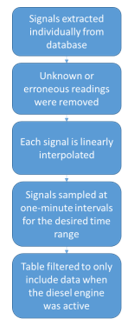Figure 1: Pre-processing steps

sampled at one-minute intervals for the desired time range, ensuring that the time range fell within the interpolated values. Finally, a filter was applied to only consider data recorded during active operation of the diesel engine.

The input parameters were standardized in order to fairly compare variables measured in different units and different ranges. The standardized variables had a mean value of zero and standard deviation equal to one.

5. Low-dimensional mappings

5.1.  Intrinsic dimension results

Estimates of the intrinsic dimension of the turbocharger data were calculated using the five techniques detailed in Section 3.1. These estimates are listed in Table 2. The first three principal components represent 0.981 of the total variance in the data.

Table 2: Intrinsic dimension estimates

Estimation Method	Estimate
Maximum Likelihood Estimator	5.239
Correlation Dimension	1.285
Geodesic Minimum Spanning Tree	4.202
Nearest Neighbour Dimension	0.307
Principal Component Analysis Eigenvalues	3.000

Almost all of the estimates fall in the range of 1 to 5. Since the original sensor space corresponds to a dimension of 31, these estimates show that the information contained in that 31-D high dimensional space could be sufficiently explained more simply by the combination of a few factors. A target dimension of 3 was selected, taking into account the range of estimates.

5.2.  Transformation to 3-dimensions

From the intrinsic dimension results, low-dimensional representations  of  the  turbocharger  data  with  three  dimensions

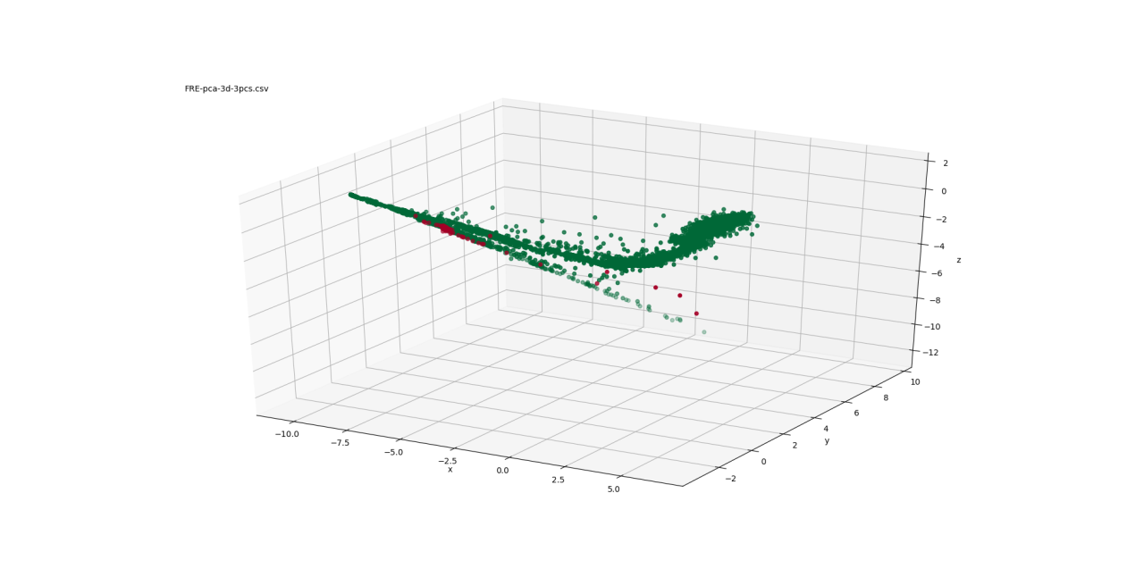
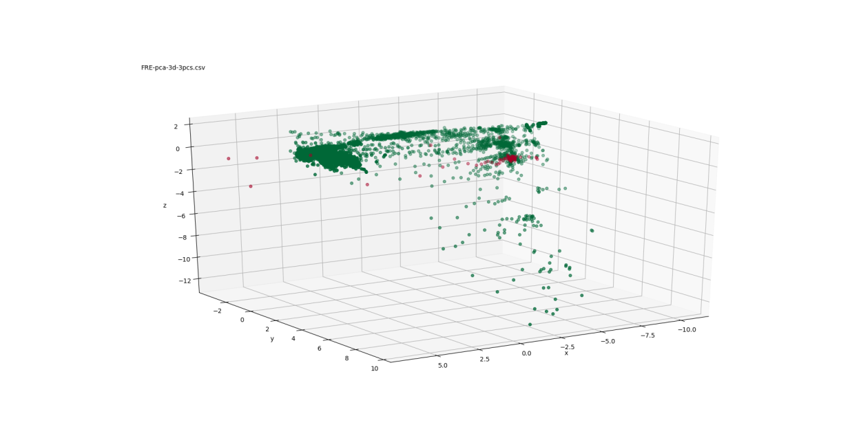
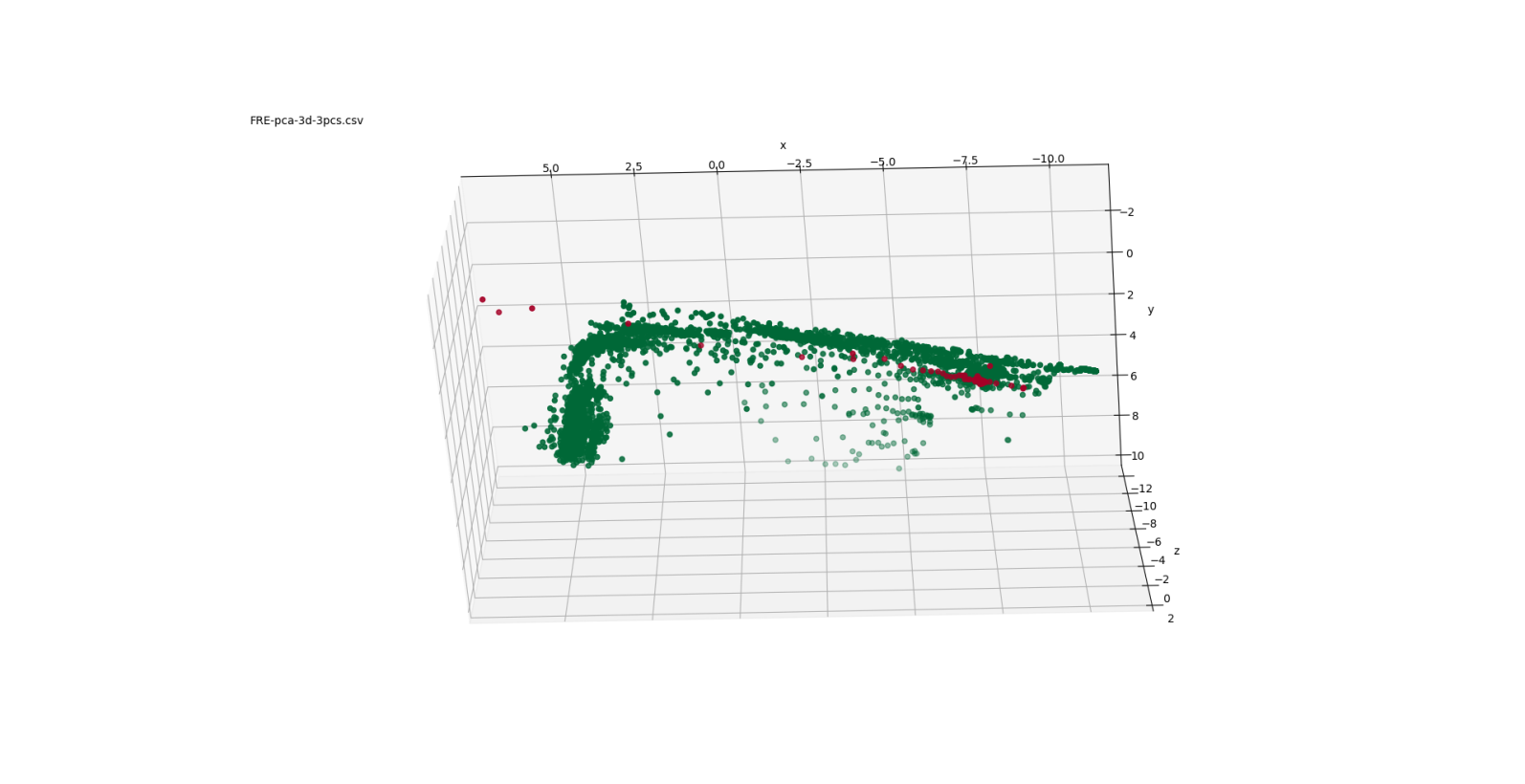Figure 2: PCA mappings to 3-D

were sought. The transformation of the original 31-D space, corresponding to the 31 turbocharger sensors, to 3-dimensions was performed using the four methods described in Section 3.2 (principal component analysis, Sammon, t-SNE, and Isomap). The full data set from the time period around the turbocharger event was mapped, consisting of 9968 total points of which 93 were designated ‘failed’ and the rest ‘healthy’.

Images of the 3-D spaces obtained from the different mappings are presented in Figures 2-5. In these images, the healthy points are coloured green, while the failed points are red. Since the ratio of healthy to failed points is tremendously imbalanced (9875:93), it may be difficult to see the failed points. Representing 3-D scenes by 2-D images is clearly not ideal because of the limitations in exploring different perspectives and distances between objects in the scene. Several snapshots of the 3-D space are included to help overcome that limitation.

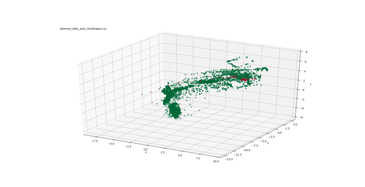
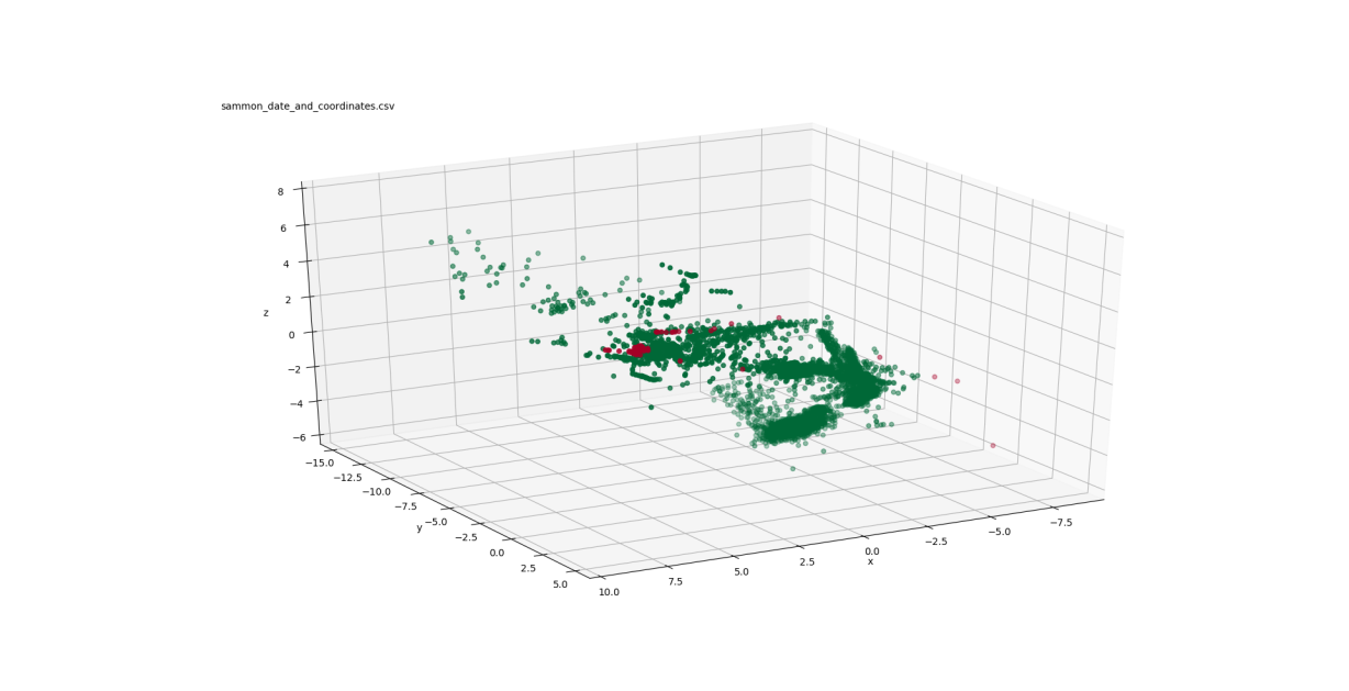
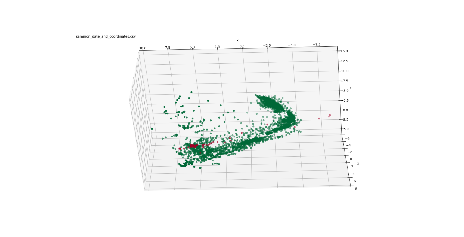Figure 3: Summon mappings to 3-D

Figure 2 shows three views of the low-dimensional mapping using the first three principal components determined through PCA. These three components are orthogonal and are linear combinations of the 31 turbocharger variables. Figure 3 depicts three views of the Sammon mapping to 3-dimensional space. Figure 4 shows the t-SNE mapping to 3-D. Figure 5 illustrates the Isomap transformation to 3-dimensions.

In the PCA mapping (Figure 2), the data is distributed mostly in a 2-dimensional plane in a boomerang-like shape. The failed points are concentrated at one end of that boomerang shape ( ). The Sammon mapping (Figure 3) also shows the distribution of the data in a boomerang-like shape. Again, the failed points are clustered at one end of that shape ( ).

The t-SNE transformation (Figure 4) has a markedly different data structure with the data organized in more distinct clusters as opposed to the continuous distribution of data in a particular shape

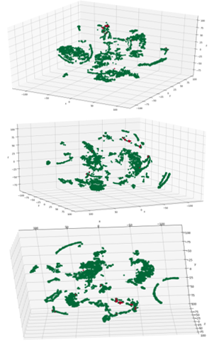Figure 4: t-SNE mappings to 3-D

(e.g. boomerang). The failed points are located in several areas of the structure in the t-SNE mapping. This is a consequence of the property expressed by the mapping (Section 3.2, t-SNE), which focuses on preserving conditional probability distributions within neighbourhoods, rather than distances. Exposing cluster structure more clearly is one of the strengths of t-SNE.

The Isomap plots (Figure 5) show a similar data structure to PCA and Sammon with much of the data falling along a boomerang-like shape. Also similar to PCA and Sammon, the failed points are all concentrated at one end of that main boomerang shape (5 ). However, more prevalent in the Isomap plot, than with the other plots, is one dense island of healthy data points just offset from that main shape, which will be discussed further in Section 6.2. The similar data structure  seen with the PCA, Sammon and Isomap plots can be attributed to the fact that nonlinear effects are mild.

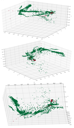Figure 5: Isomax mappings to 3-D

The transformation of the 31-dimension space representing the 31 turbocharger parameters to a low-dimensional 3-D space shows a distinct data structure in the various mapping techniques. The failed points are not mapped to an obvious outlier location in the transformations that can be easily distinguished from the healthy points.

6. Relating sensor signals to internal data structure

In order to better understand these data structure visualizations in a more physical sense, e.g. from the perspective of the operator or maintainer of the engine, the next step was to select a handful of the engine signals and examine how each of these signals impacted and was represented in the data structure. One of the aims was to determine if certain regions of the mappings could be associated with distinct operational states of the engine. Another aim was to demonstrate that individual signals were appropriately represented in the low-dimensional mapping.

6.1.  Selected signals

As detailed in Table 1, a variety of sensors recording speeds, temperatures, pressures and torque were included in the analysis. A small subset of signals was selected to investigate the internal data structure of the mappings. The selected signals were: Turbo A speed, Turbo B speed, A1 cylinder exhaust gas temperature, B2 cylinder exhaust gas temperature, and engine speed.

As there was a known failure of the Turbo A speed signal, the Turbo B speed signal was selected to compare the recorded values of the two turbos. In a similar manner, at the time of failure, the exhaust cylinder temperature sensors went into alarm. To enable comparison of the exhaust temperatures, one cylinder exhaust temperature signal was selected from each bank. Finally, engine speed was selected, although it was not part of the 31 turbocharger parameters used for the transformations. This sensor was included as it is the main driving factor for change in the values of the other sensor signals.

6.2.  Representation of signals in low-dimensional mappings

Each of the low-dimensional mappings was then overlaid with a heat map of one of these sensor signals. Where instead of the data points coloured green and red for healthy and failed points respectively, they were coloured according to the relative value of the particular signal in its operating range, with blue corresponding to the low end of the range and red for the high end of the operating range.

In the following section of the paper, two regions of interest are highlighted: i) the points surrounding the time frame where the Turbo A speed sensor experienced a fault and failed to record; and ii) the points surrounding the five minutes to the turbocharger seizure.

These two regions were chosen for further investigation because they appear to stand out the most in the visualizations. The Isomap low-dimensional mappings are shown in this paper with an overlay of the  heat  map  for  the  five  selected  signals.  Figure 6

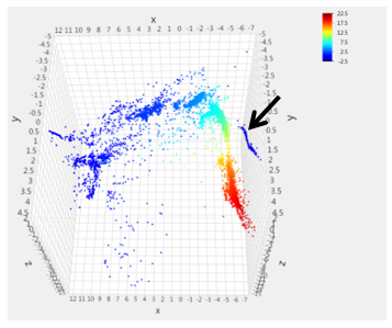Figure 6: Turbo A speed sensor value [kRPM] overlay onto Isomap transformation

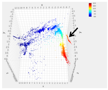Figure 7: Turbo B speed sensor value [kRPM] overlay onto Isomap transformation

shows the overlay of the Turbo A speed signal on the Isomap transformation. Figure 7 shows the overlay of the Turbo B speed signal on the Isomap transformation. Since both these signals are speed sensors on turbochargers, the expectation is that these two plots should be very similar. For the most part the two plots are indeed very similar, however, it should be noted that the speed ranges are slightly different in the legend.

The distribution of the data points in the mapping indicates that almost all the near-zero/low-speed data points are found in one region of the data structure ( ) while the data points with high speed values are concentrated in a different region ( ). There is a strong gradient between these two regions containing a transition region of the intermediate speeds.

However, an abnormality to the general structure of the data is evident in the high power region of the plots. In Figure 6, the heat map indicates zero values for the Turbo A speed sensor for the data points in the area indicated by the arrow. In the same area, indicated by the arrow in Figure 7, the Turbo B speed sensor portrays high speed values. The overlays of the other examined signals displayed expected values for those data points in that high power region. Thus this group of points is likely related to the loss of the Turbo A speed sensor. Indeed the data points in this area were later found to coincide with the known initial loss of the Turbo A speed sensor readings.

Figure 8 shows the overlay of the Turbo A Cylinder 1 exhaust gas temperature signal on the Isomap transformation. Figure 9 shows the overlay of the Turbo B Cylinder 2 exhaust gas temperature signal on the Isomap transformation. Figure 10 shows the overlay of engine speed signal on the Isomap transformation. The plots of the two cylinder exhaust temperatures from each bank (Figures 8 and 9) are quite similar to each other, as one would expect. They are also structured similar to the Turbo speed overlays where the data points with low temperature values also have low speed values, while the high temperature points have high speed values.

Figure 8: Turbo A Cylinder 1 exhaust gas temperature [˚C] overlay onto Isomap transformation

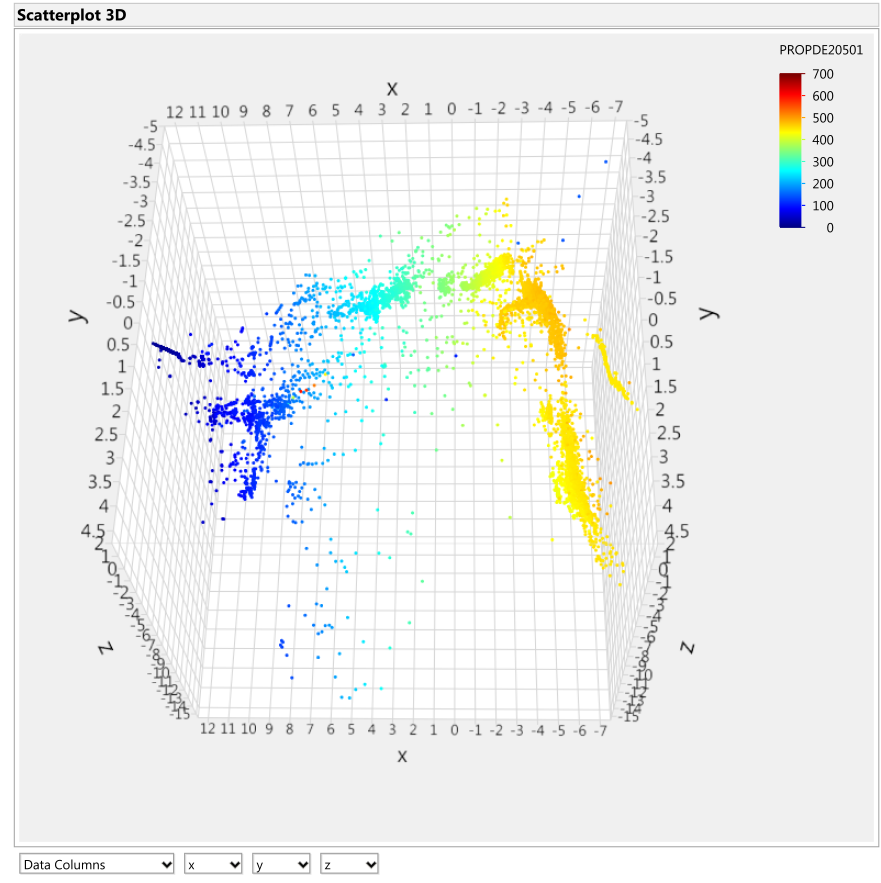Figure 9: Turbo B Cylinder 2 exhaust gas temperature [˚C] overlay onto Isomap transformation

A small cluster of high cylinder temperature indications is found within the low operating range group indicated by the purple circle in Figures 8 and 9. These points were later found to be the points occurring five minutes before the turbocharger seizure. The location of these points in the low speed range is consistent with the findings of the turbocharger incident report (described in Section 2), where an increase in speed was requested but no increase in speed was realized although the exhaust gas temperatures rose to high levels invoking the alarms.

Although engine speed was not a signal used to generate the Isomap transformation, here it is used as a means to support the previously observed trends of low and high operating ranges in the plots. From Figure 10, the engine speed overlay demonstrates a similar distribution of the low and high engine  speeds in  the data

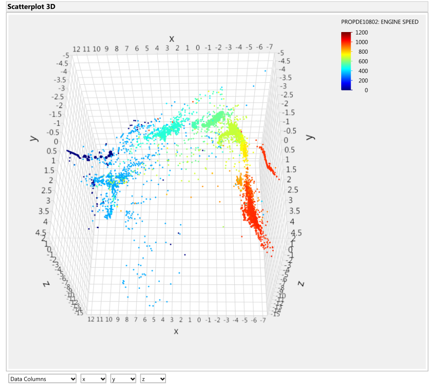Figure 10: Engine speed [RPM] overlay onto Isomap transformation

structure. Looking again at the data points indicated by the arrow in Figure 10, the trend seen previously with the Turbo speeds and cylinder exhaust temperatures is confirmed.

According to Figure 5, the data points indicated by the arrow in the prior figures are clearly distant from the main set of data and are still designated as ‘healthy’. It was also pointed out that the small cluster of cylinder exhaust gas temperature indications (some of the points inside the region of the purple circle in Figures 8 and 9) represent values that were recorded between five hours and five minutes to the turbocharger seizure. These points embed themselves inside low operating ranges of these signals and are also designated as ‘healthy’ data (Figure 5). In both cases, the aforementioned groups of points display interesting traits through the unique combination of their healthy/failed designation, the value of the overlaid signal that they show, and their distance from other groups of data points. This demonstrates that the failure of the turbocharger system may not always be associated with extreme signal values, as one may assume. These traits help uncover new trends in the data structure, like the abnormality indicated by the arrow or the cluster of points within the purple circle in the preceding figures, which should be investigated. Thus, being able to combine expert domain knowledge of sensors and failures with data mining tools is an invaluable method of extracting and understanding information from sensor measurements.

7. Concluding Remarks

This work describes continued analysis of sensor data for the turbocharger subsystem of a diesel engine system. The engine has hundreds of sensors monitoring both the inputs of the engine operator and the resulting equipment outputs. The objective of the data analysis was to characterize and distinguish the healthy and failed states of the turbocharger seizure as recorded by the diesel engine sensor system. The analysis approach included the mapping of high-dimensional sensor data to a low-dimensional space using a variety of linear and nonlinear techniques in order to highlight and visualize the underlying structure of the information.

Estimates of the intrinsic dimension were obtained to determine the appropriate number of dimensions required by the low-dimensional transformations and to guide the interpretation of the visualization spaces produced. For this case, three dimensions was an appropriate estimate. Through the unsupervised process of these transformations, the structure of the turbocharger data could be visualized and inspected. The transformation methods included principal components, Sammon mapping, t-Distributed Stochastic Neighbour Embedding, and Isomap. The transformation of the 31-dimension space representing the 31 turbocharger parameters to a low-dimensional 3-D space shows a distinct data structure in the various mapping techniques. The failed points are not mapped to an obvious outlier location in the transformations that can be easily distinguished from the healthy points.

In order to gain more physical insight into the internal data structure of the resulting mappings, the transformation plots were analyzed from the perspective of several engine sensor signals. By overlaying operating ranges of individual sensor signals, certain regions of the mappings could be associated with distinct operational states of the engine. Low and high operating engine regions could be clearly seen in the internal data structure, and several anomalies could be identified which were then associated to various points in the turbocharger seizure. These results are extremely promising and demonstrate how operational knowledge can be easily incorporated with the data analytics tools to enhance the insights that can be gained from the sensor measurements.

In this work, data mining and machine learning techniques are implemented to gather useful insights from the large amounts of sensor data collected for this diesel engine system. By incorporating expert domain knowledge with the low-dimensional representations of the data, a more practical understanding of the data structure presented in the mappings is provided which helps ensure that the results are relevant and accessible to the operator and end-user.

Future efforts are aimed at expanding this analysis to data from other diesel engines and other failures in the engine system. Further work to generalize the analysis to a diesel engine system model instead of a turbocharger-specific model is in progress. Efforts are also underway to better characterize the healthy and failed states, through classification and anomaly detection techniques. The development and implementation of these tools should help enable advance indication of a change in behavior that could be investigated before a major incident.

Conflict of Interest

The authors declare no conflict of interest.

Acknowledgment

The authors would like to acknowledge and thank Defence Research and Development Canada for their support of this research.

1.  C. Cheung, J. J. Valdés, A. Lehman Rubio, R. Salas Chavez, C. Bayley, “Low-dimensional spaces for the analysis of sensor network data: identifying behavioural changes in a propulsion system” in 5th International Symposium on Robotics and Intelligent Sensors, Ottawa, Canada, 2017. https://www.doi.org/10.1109/IRIS.2017.8250133
2.  A. Widodo, B. Yang, “Support vector machine in machine condition monitoring and fault diagnosis” Mech. Syste. Signal Pr., 21(6), 2560-2574, 2007. https://www.doi.org/10.1016/j.ymssp.2006.12.007
3.  S. Li, “Induction motor fault diagnosis based on fuzzy support vector machine” in 3rd International Conference on Electromechanical Control Technology and Transportation, 2018. https://www.doi.org/10.5220/0006975105880592
4.  M. Saimurugan, K. Ramachandran, V. Sugumaran, N. Sakthivel, “Multi component fault diagnosis of rotational mechanical system based on decision tree and support vector machine” Expert Syst. Appl., 38(4), 3819-3826, 2011. https://www.doi.org/10.1016/j.eswa.2010.09.042
5.  M.C. Garcia, M.A. Sanz-Bobi, J.D. Pico, “SIMAP: intelligent system for predictive maintenance” Comput. Ind., 57(6), 552-568, 2006. https://www.doi.org/10.1016/j.compind.2006.02.011
6.  U. Fayyad, G. Piatetsky-Shapiro, P. Smyth, “From data mining to knowledge discovery in databases” AI Mag., 17(3), 1996. https://doi.org/10.1609/aimag.v17i3.1230
7.  C. Torrano-Gimenez, H.T. Nguyen, G. Alvarez, K. Franke, “Combining expert knowledge with automatic feature extraction for reliable web attack detection” Secur. Commun. Netw., 8, 2750–2767, 2015. https://www.doi.org/10.1002/sec.603
8.  F. Kuusisto, I. Dutra, M. Elezaby, E.A. Mendonça, J. Shavlik, E.S. Burnside, “Leveraging expert knowledge to improve machine-learned decision support systems” AMIA Jt Summits Transl Sci Proc, 87–91, 2015.
9.  J. Valdés, C. Y. S. Létourneau, “Data fusion via nonlinear space transformations” in 1st International Conference on Sensor Networks and Applications, San Francisco, USA, 2009.
10.  K. Fukunaga, Introduction to Statistical Pattern Recognition, Academic Press Professional Inc., 1990.
11.  E. Facco, M. d’Errico, A. Rodriguez, A. Laio, “Estimating the intrinsic dimension of datasets by a minimal neighborhood information” Sci. Rep.-UK, 7(1), 2017. https://www.doi.org/10.1038/s41598-017-11873-y
12.  D. Granata, V. Carnevale, “Accurate estimation of the intrinsic dimension using graph distances: Unraveling the geometric complexity of datasets” Sci. Rep.-UK, 6(1), 2016. https://doi.org/10.1038/srep31377
13.  P. Campadelli, E. Casiraghi, C. Ceruti, A. Rozza, “Intrinsic dimension estimation: Relevant techniques and a benchmark framework” Math. Probl. Eng., 2015. https://doi.org/10.1155/2015/759567
14. E. Levina, P. J. Bickel, “Maximum likelihood estimation of intrinsic dimension” in 17th Conference in Neural Information Processing Systems, Vancouver, Canada, 2004.
15.  P. Grassberger, I. Procaccia, “Measuring the strangeness of strange attractors” Physica D, 9(1-2), 189-208, 1983. https://www.doi.org/10.1016/0167-2789(83)90298-1
16.  J.A. Costa, A.O. Hero, “Geodesic entropic graphs for dimension and entropy estimation in manifold learning” IEEE T. Signal Proces., 52(8), 2210–2221, 2004. https://www.doi.org/10.1109/tsp.2004.831130
17.  K. Pettis, T. Bailey, A. Jain, R. Dubes, “An intrinsic dimensionality estimator from near-neighbor information” IEEE T. Pattern Anal., 1(1), 25-37, 1979. https://www.doi.org/10.1109/tpami.1979.4766873
18.  W. Press, S. Teukolsky, W. Vetterling, B. Flannery, Numerical Recipes in C, Cambridge University Press, 1992.
19.  J. Kruskal, “Nonmetric multidimensional scaling: a numerical method” Psychometrika, 29(2), 115-129, 1964. https://www.doi.org/10.1007/bf02289694
20.  J. Kruskal, “Multidimensional scaling by optimizing goodness of fit to a nonmetric hypothesis” Psychometrika, 29(1), 1-27, 1964. https://www.doi.org/10.1007/bf02289565
21.  I. Borg, P. Groenen, Modern multidimensional scaling – theory and applications, Springer Series in Statistics, 1997.
22.  I. Borg, P.J.F. Groenen, P. Mair, Applied Multidimensional Scaling, Springer Verlag, 2013.
23.  J. W. Sammon, “A nonlinear mapping for data structure analysis” IEEE T. Comput., 18(5), 401-409, 1969. https://www.doi.org/10.1109/tc.1972.5008933
24.  G. Hinton, S. Roweis, “Stochastic neighbor embedding” Adv. Neur. Inf. Proc. Systems, 15, 857-864, 2003.
25.  L. van der Maaten, G. Hinton, “Visualizing data using t-sne” J. Mach. Learn. Res., 9, 2579-2605, 2008.
26.  M. Nguyen, S. Purushotham, H. To, C. Shahabi, “M-tsne: a framework for visualizing high-dimensional multivariate time series”, University of Southern California, 2017. https://arxiv.org/abs/1708.07942
27.  J. Tenenbaum, V. de Silva, J. Langford, “A global geometric framework for nonlinear dimensionality reduction” Science, 290(5500), 2319-2323, 2000. https://www.doi.org/10.1126/science.290.5500.2319
28.  M. Bernstein, V. de Silva, J. Langford, J. Tenenbaum, “Graph approximations to geodesics on embedded manifolds” Stanford University, Tech. Rep., 2000.
29.  V. de Silva, J. Tenenbaum, “Global versus local methods in nonlinear dimensionality reduction” Adv. Neur. Inf. Proc. Systems, 15, 721-728, 2003.
30.  H. Choi, S. Choi, “Robust Kernel Isomap” Pattern Recogn., 40(3), 853-862, 2007. https://www.doi.org/10.1016/j.patcog.2006.04.025

(Click Here)

(Click Here)