1. Introduction

MMACS algorithm is a hybrid metaheuristic that was proposed in a previous work [1] and employed to solve one of the most complex variants of the knapsack problem which is the Strongly Correlated Knapsack Problem (SCKP). The proposed approach combines a proposed Ant Colony Optimization algorithm (ACO) with a 2-opt algorithm. The proposed ACO scheme combines two ant algorithms: the MAX-MIN Ant System and the Ant Colony System. At a first stage, the proposed ACO aims to solve the SCKP to optimality. In case an optimal solution is not found, a proposed 2-opt algorithm is used. Even if the 2-opt heuristic fails to find the optimal solution, it would hopefully improve the solution quality by reducing the gap between the found solution and the optimum. An optimal resolution of a combinatorial optimization problem by applying an approximate method requires an adequate balance between exploitation of the best available solutions and wide exploration of the research space. On the one hand, the aim of exploitation is to intensify the research around the most promising areas of the research space, which are in most cases close to the best-found solutions. On the other hand, it comes to diversifying the research by encouraging the exploration in order to discover new and better areas of the research space. The behavior of ants in relation to this duality between exploitation and exploration can be affected by the adjustment of the parameter values.

A comparative study was conducted on the hybrid ant colony algorithm MMACS. Firstly, this study is intended to present the behavior of MMACS algorithm and its dependencies on the values given to parameters while solving SCKP. Secondly, a comparison of performances of MMACS algorithm and two well-known Ant Colony Algorithms: the Max-Min Ant System (MMAS) and the Ant Colony System (ACS) was provided. Finally, MMACS algorithm was compared with two recent state of art algorithms that show significant results when solving the SCKP to optimality. The paper has been organized as follows. In the next section, we define the Strongly Correlated Knapsack Problem. We present the studied Ant Colony Optimization algorithms (ACO) in section 2. In section 3, we introduce the parameters in ACO. Then, we define the local search in section 4. Finally, experiments and results are presented in section 5.

2. Strongly Correlated Knapsack Problem (SCKP)

The SCKP problem is a NP-hard problem, whose goal is to find a subset of items that maximizes an objective function while satisfying resource constraints. In SCKP, the profit of each item is linearly related to its weight, in other words, the profit of an item is equal to its weights plus a fixed constant. The complexity of this problem compared to the classical knapsack problem resides in the strong correlation between the variables that characterize the problem. According to Pisinger in [2], the strongly correlated instances are hard to solve for two reasons. First, they are badly conditioned in the sense that there is a large gap between the continuous and integer solution of the problem. Then, sorting the items according to decreasing efficiencies corresponds to a sorting according to the weights. Thus, for any small interval of the ordered items (i.e. a ”core”), there is a limited variation in the weights, making it difficult to equally satisfy the capacity constraint. SCKP can be formulated as follows:

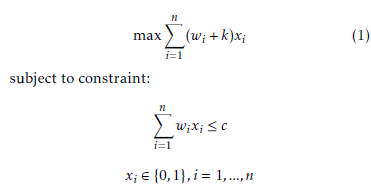where x_i is a decision variable associated with an item i, which has value 1 if the item is selected and 0 otherwise, w_i is the weight of the item i uniformly random [1,R], k is a positive constant, c is the knapsack capacity and n is the number of items. The capacity of the knapsack c is proposed by Pisinger in [2] and it is obtained as follows :

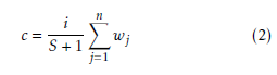where S is the series of instances as such, for each instance, a series of S = 100 instances is performed and i = 1,..,S corresponds to the test instance number. From equation (1), the profit prof it(x) of a solution x

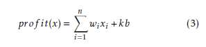where b is the number of items in x. According to equation (3), the maximization of the prof it(x) means the maximization of the number of the selected items. In other words, items with the lowest weights should be first selected until the sum of weights is about to exceed the capacity c. This can be achieved through the use of greedy algorithms [3, 4]. However, greedy does not guarantee optimal solutions since it chooses the locally most attractive item with no concern for its effect on global solutions. The convergence to local optima caused by greedy algorithms, called stagnation, should be avoided, hence the idea of alternation between greedy and stochastic approaches.

The proposition of Pisinger in [5] is one of the most well-known works that shows significant results when solving the SCKP to optimality. Pisinger proposed a specialized algorithm for this problem where he used a surrogate relaxation to transform the problem into a Subset-sum problem. He started the resolution by applying a greedy algorithm, then he used a 2-optimal heuristic and a dynamic programming algorithm to solve the problem to optimality. More recently, Han [6] proposed an evolutionary algorithm inspired by the concept of quantum computing. The study in [6] shows that the proposed algorithm, called Quantum-Inspired Evolutionary Algorithm (QEA), can find high quality results when solving the strongly correlated knapsack problems.

3. Ant Colony Optimization (ACO)

The ACO [7, 8] is a constructive population-based metaheuristic inspired from the real ants’ behavior, seeking an adequate path between their colony and a food source, which is often the shortest path. The communication between ants is mediated by trails of a chemical substance called pheromone. Several ant colony optimization algorithms have been proposed in the literature. In this section, we present the MaxMin Ant System proposed by Stutzle and Hoos [¨ 9, 10], the Ant Colony System proposed by Gambardella and Dorigo [11] and a recent hybrid ant colony algorithm called MMACS.

3.1. MMAS

The Max-Min Ant System [9, 10] is one of the most effective solvers of certain optimization problems. In MMAS, ants apply a random proportional rule to select the next item. The probabilistic action choice rule is defined as follows:

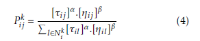where τ and η are successively the pheromone factor and the heuristic factor, α and β are two parameters that determine the relative influence of the pheromone trail and the heuristic information and N_i^k is the feasible neighborhood of an ant k that selected an item i and chooses to select an item j. Besides, MMAS exploits the best solutions found by letting only the best ant deposit pheromone. This best ant can be the one which found the best solution during the last iteration or the one which found the solution from the beginning of the execution. The pheromone update can be formulated as follows:

1. Pheromone evaporation applied to all components:

2. Pheromone update applied to components selected by the best ant:

Then, MMAS introduces bounds to limit the range of pheromone trails to [τ_min,τ_max] in order to escape a stagnation that can be caused by an excessive growth of pheromone trails. These pheromone trails are initialized, at the beginning, to upper pheromone trail limit to ensure the exploration of the research space, and reinitialized when system approaches stagnation.

3.2. ACS

The ACS algorithm [11] achieves performance improvement through the use of a more aggressive action choice rule. In ACS, ants choose items according to an aggressive action choice rule called pseudorandom proportional rule given as follows:

argmax

where q is a random variable uniformly distributed in [0,1], q₀ (0 ≤ q₀ ≤ 1) and S is a random variable selected according to the probability distribution given in equation (4). Besides, only one ant called the bestso-far-ant is allowed to deposit pheromone after each iteration. Thus, the global pheromone trail update is given as follows:

This pheromone trail update is applied to only components in the best-so-far solution, where the parameter ρ represents pheromone evaporation. In addition to the global pheromone update, ants use a local pheromone update rule that is applied immediately after choosing a new item during the solution construction, given as follows:

where 0 <  < 1 and τ₀ are two parameters such that the τ₀ value is equal to the initial value of the pheromone trails which is 0.1. The local update happens during the solution construction in order to prevent other ants to make the same choices. This increases the exploration of alternative solutions.

3.3. MMACS

The MMACS algorithm combines Max-Min Ant System with Ant Colony System and an algorithm based on the 2-opt heuristic. In fact, the scheme of MMACS is based on ACO scheme presented in [12] and ACS scheme presented in [11] in a way that it uses an MMAS pheromone update rule and a choice rule inspired from the ACS aggressive action choice rule. In MMACS, the minimum and the maximum pheromone amounts are limited to an interval [τ_min,τ_max], like MMAS, in order to avoid premature stagnation. Initially, the pheromone trails are set to τ_max. After the construction of all solutions in one cycle, the best ant updates the pheromone trails by applying a rule similar to MMAS pheromone update rule. Indeed, once all ants finish the solutions construction, the pheromone trails are decreased to simulate evaporation by multiplying each component by a pheromone persistence ratio equal to (1 − ρ) where 0 ≤ ρ ≤ 1 as given by equation (5). After that, an amount of pheromone is laid on the best solution found by ants by applying the pheromone update rule given in equation (6), where the amount of pheromone trails is calculated as follows:

S_best represents the best solution built since the beginning and S_k is the best solution of a cycle. Besides, in MMACS, each ant constructs a solution by applying the choice rule, where the decision making is based on both:

1. A random proportional rule that selects a random item using the probability distribution.
2. A guided selection rule that chooses the next item as the best available option.

Like ACS, MMACS balances between greedy and stochastic approaches by applying the pseudorandom proportional rule (7). Actually, at each construction step, an ant k chooses a random variable q uniformly distributed in [0,1]. If q is less than a fixed parameter q₀ such as 0 ≤ q₀ ≤ 1, the ant makes the best possible choice as indicated by the pheromone trails and the heuristic information (exploitation) else, with a probability 1 − q₀ , the ant applies the random proportional rule (4) to select the next item (biased exploration). The heuristic factor used in the probability rule (4) is given as follows:

where d_Sk is the remaining capacity when an ant k built a solution S_k and it is given as follows:

As shown in equation (11), the heuristic information value and the item weight are inversely proportional. Consequently, the more the weight value decreases the more the heuristic information value increases. Added to that, the closer the remaining capacity and the item weight are, the more the heuristic information value increases. This can be helpful at the end of the execution when the knapsack is about to be filled. At last, the execution of MMACS algorithm ends either when an optimum is found, or in the worst cases, it ends after a fixed number of iterations. The pseudocode of MMACS algorithm is represented by algorithm 1.

Algorithm 1 MMACS pseudo-code applied to SCKP

Initialize pheromone trails to τ_max repeat

repeat

Construct a solution Update S_best until maximum number of ants is reached or op-

timum is found

Update pheromone trails until maximum number of cycles is reached or optimum is found

Apply a local search algorithm

S_best is the best solution found all along the execution.

The construction procedure can be represented by algorithm 2.

Algorithm 2 Construct Solution

Select randomly a first item

Remove from candidates each item that violates resource constraints while Candidates , Ø do

if a randomly chosen q is greater than q₀ then Choose item o_j from Candidates with probability Pijk else

Choose the next best item end if

Remove from candidates each item that violates

resource constraints

end while

4. Parameters in ACO

In the ACO algorithm, relevant parameters that request reasonable settings are the heuristic information parameter β, the pheromone parameter α and the pheromone evaporation rate ρ. Those parameters can influence the algorithm performance by improving its convergence speed and its global optimization ability.

4.1. The heuristic information parameter β

The ants’ solution construction is biased by a heuristic value η that represents the attractiveness of each item.

The parameter β determines the relative importance of this heuristic value. In our case, the heuristic information makes items characterized by little weights as desirable choices. In other words, the increase in the β value can be triggered by the selection of items which have little weights. This behavior is close to that of greedy algorithm. However, the decrease in the value of β makes the heuristic factor unprofitable. As a result, ants fall easily in local optima.

4.2. The pheromone parameter α

Besides heuristic value, the ants’ solution construction is influenced by the pheromone trails. The pheromone parameter α determines the relative influence of the pheromone trails τ. Indeed, the parameter α reflects the importance of the amplification of pheromone amounts. In other words, the increase of α favors the choice of items associated with uppermost pheromone trails values. In case the value of α is considerable, ants tend to choose the same solution components. This behavior is caused by the strong cooperation between them so ants drift towards the same part of the search space. In such case, the convergence speed of algorithm accelerates and consequently, it causes the fall in local optima. This gives rise to the need to prevent this premature convergence. Then, several tests were conducted to evaluate the influence of α on solutions’ quality. Additional experiments were carried out to examine the similarity of solutions in one cycle. The analysis of the similitude of solutions allows appropriately assigning the value of α in order to avoid the premature stagnation of the search that can be caused by the excessive reliance upon pheromone trails at the expense of the heuristic information.

4.3. The pheromone evaporation rate ρ

The amount of pheromone decreases to simulate evaporation by multiplying each component by a constant evaporation ratio equal to 1 − ρ. This pheromone trails reduction gives ants the possibility of abandoning bad decisions previously taken. In fact, the pheromone value of an unchosen item decreases exponentially with the number of iterations.

5. Local search

Table 1: Default parameter settings for MMAS, ACS and MMACS algorithms ACO algorithm α β ρ ants cycles q0 MMAS 1 2 0.02 n 20 MMAS + 2-opt 1 2 0.2 25 20 ACS 2 0.1 10 20 0.9 ACS + 2-opt 2 0.1 10 20 0.98 MMACS 1 5 0.02 20 20 0.9

Local search algorithms are usually used in most applications of ACO to combinatorial optimization problems in order to improve solutions found by ants. Among those algorithms, we cite 2-opt heuristic. The 2-opt [13] is a simple local search algorithm. When applied to knapsack problems, it consists of exchanging an item present in the current solution with another that is not part of this solution in order to improve it. The new solution should satisfy constraints and it would be better or equal to the old one. In other words, the 2-opt algorithm takes a current solution as input and returns a better accepted solution to the problem, if it exists. The 2-opt algorithm is used once the ants have completed their solution construction, thereby improving the solution by approaching the best one or even reaching it. Our proposed 2-opt algorithm can be written as represented by algorithm 3.

Algorithm 3 A 2–opt pseudo-code applied to SCKP

Initialize Candidates by observing S_best repeat

for each item o_j ∈ Candidates do

for each item o_i ∈ S_best do

                 Sbest0    = Swap (oi, oj)                       0                       0

if constraints are satisfied by S_bestand S_best is

better than S_best then

Update best solution end if end for

end for

until no improvement is made

6. Computational results

In this section, we study the results of a set of experiments that was carried out to determine the efficacy of the MMACS algorithm. The proposed algorithm was programmed in C++, and compiled with GNU g++ on an Intel Core i7-4770 CPU processor (3.40 GHz and 3.8 GB RAM).

Through the experimentations, we analyze the influence of the parameters’ selection on the MMACS performances. Then, we identify the convenient parameter settings that produce better results. Those parameter settings are employed for the rest of the experiments. At a later stage, we compare the results of MMACS with those of the two well-known ant colony algorithms: MMAS [9, 10] and ACS [11]. After that, the results of MMACS are compared with those of the evolutionary algorithm QEA in [6] and to the optimal values.

6.1. Benchmark instances

In order to evaluate the performance of the MMACS algorithm, experiments were conducted on two sets of instances.

6.1.1. Pisinger Set

The first set contains 100 different instances with n items, where the number of items n varies from 50 to 2000. Those benchmark instances used in comparison with algorithms in [5] and [6] are available at the website (http://www.diku.dk/pisinger/codes.html).

6.1.2.  Generated Set

The second set regroups 3 different instances having the number of items equal to 100, 250 and 500, respectively. Those instances used in comparison with the proposed algorithm in [6], were randomly generated using a generator similar to the one in [2].

6.2. Parametric analysis of MMACS

In order to evaluate the influence of parameters’ values on MMACS performances, we conducted tests for different values of parameters and compared the obtained results. The experiments were realized on the Pisinger set instances of size 50, 100, 200 and 500, and for each instance, we applied 10 runs (10 runs * 100 instances * 4 knapsack problems). In each of these experiments, we fixed the parameters to their default values and we made the variation of the studied parameter. In fact, the MMAS and ACS default parameter settings were recommended by the authors in [14]. The default parameter settings are given in Table 1 and the various values for each parameter are presented in Table 2. Tables 3- 29 report the results of MMACS algorithm in response to the variation of the parameters. N is the number of items and R is the range of coefficients. Then, the presentation of the data is visualized using different curves. Figures 1- 5 present the effect of the studied parameters on MMACS performances. The abscissa axis of curves presented in those figures shows the instances’ size that varies between 50 and 500. In each figure, left and right plots show the behavior of MMACS algorithm while solving the SCKP instances having the range of coefficients equal to 1000 and 10000, respectively. In those curves, we examine the percentage of exact solutions, the relative deviation of the best solution found by MMACS from the optimal solution value and the execution time in terms of the studied parameter.

Table 2: Parameter settings used in experiments for

MMACS algorithm

Control parameter	Value
α	1, 2, 3, 4, 5
β	1, 2, 3, 4, 5
ρ	0.01, 0.02, 0.4, 0.5, 0.8, 1
q0	0, 0.5, 0.75, 0.9, 0.99
m	1, 5, 10, 20, 50, 1000

6.2.1. Influence of parameter α

We set the value of β to 5 and ρ to 0.02. After that, we make the change of the value of α in order to study its influence on the solutions’ quality and the execution time. Tables 3- 6 represent the results after applying MMACS to SCKP where α varies between 1 and 5. Results are visualized using curves in Figure 1. In fact, the differences among the various settings of α are almost insignificant. However, the value of α equal to 1 gives better results in terms of the most reduced execution time. Additional experiments are conducted to analyze the similitude of solutions in one cycle in order to appropriately assign the value of α. In fact, we propose to calculate a similarity ratio proposed in [15]. The similarity ratio associated with a set of solutions S is defined as follows:

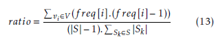where V is a set of items and f req[i] is the frequency of the object v_i in the solutions of S. Thus, this ratio is equal to 1 if all the solutions of S are identical and it is equal to 0 if the intersection of solutions of S is empty. In those experiments, the number of cycles varies from

10 to 25. For each number of cycles, each ant’s solution was compared with others. Experiments are conducted on the Pisinger set instances of size 100 and for both range of coefficients 1000 and 10000. Figure 2 shows the influence of the pheromone trails on the similarity of the solutions built during the execution of the MMACS algorithm, and for different values of the α parameter that determine the influence of the pheromone on the behavior of the ants. The curves show that the solutions are remarkably similar where the similarity ratio varies between the values 0.6 and 0.8 beginning with the number of cycles at about 15. In other words, ants are not deeply influenced by pheromone trails and they are obviously focusing in a short time on a very small area of the research space that they explore intensely.

6.2.2. Influence of parameters β and ρ

In this section, we examine the influence of different values of the heuristic information parameter β and the pheromone evaporation rate ρ. In this context, we fix the value of α to 1 then we make a simultaneous variation of the two variables β and ρ. We modify the values of β in order to control the influence of the heuristic information and to examine its effect on the MMACS performances. Besides, we make the variety of ρ values in order to study its influence on the items’ selection and consequently on the MMACS performances. Tables 7- 21 present results after applying MMACS to SCKP where β varies between 2 and 5 and ρ values are 0.01, 0.02, 0.4, 0.5, 0.8 and 1.

Results of MMACS algorithms with the fixed parameter β are almost similar to all values of ρ.

The MMACS algorithms with the fixed parameter β1 and β2 work in a similar way. In fact, the results show that the percentages of exact solutions decrease considerably in terms of number of items for both ranges of coefficients 1000 and 10000. Consequently the values of gap increases. Besides, the execution time results vary in the same way for the six values of ρ.

The MMACS algorithms with the fixed parameter β3 and β4 behave in a similar way for almost all problems with both ranges of coefficients 1000 and 10000. Results show that the percentages of exact solutions for both algorithms increase for number of items between 50 and 200. Then these percentages decrease considerably for the large number of items 500. Consequently, the gap results progress in a reverse way.

However, the MMACS algorithm with the fixed heuristic parameter β5 shows acceptable results. Results are presented in Figure 3, each curve represents a value of ρ. The curves have almost the same evolutions with insignificant differences between the values. In fact, the percentage of exact solution presents an increase in terms of number of items. Besides, the gap results show a remarkable decrease for large instances. Then, the execution time has the same variation for all values of ρ.

However, the value of ρ2 equal to 0.02 selected by MMACS can be modified to ρ1 in order to make a slight improvement in gap values for large instances with a range of coefficients equal to 10000.

6.2.3. Influence of parameter q₀

In MMACS, we study the effect of q₀ that represents the probability of selecting the best available choices in equation 7. Results are given in Tables 22- 25 and presented in curves of Figure 4. The curves in Figure 5 are associated with the values of q₀: 0, 0.5, 0.75, 0.9 and 0.99. For all instances, among those values only 0.9 and 0.99 show an increase in terms of the percentage of the exact solutions. As regards the other values of q₀ MMACS does not succeed in finding, in most cases, the exact solution. This is clearly represented by its decreasing curves. As to the execution time, the five curves are growing in almost the same way. However, the curve that corresponds to q₀ value equal to 0.9 reaches the lowest values. For large instances, the differences between the curves are significant. The best results that correspond to the lowest gap values is represented by the curve associated to the value of q₀ equal to 0.9. We conclude that MMACS has the same behavior as ACS regarding the q₀ parameter, where the values close to 1 present the good ones as suggested in the literature.

6.2.4. Influence of colony size

Tables 26- 29 show the effect of colony size on the quality of the solutions. In these tables, the ant colony size m varies between 1 and 100. Results are compared in Figure 5. As shown by curves in Figure 5, the increase in the ants’ number improves the percentage of exact solutions. This increase causes the growth of the execution time, although in practice, we generally seek to

Table 3: Percentage of exact solutions found by MMACS. The value of α varies between 1 and 5.

N	R	α1	α2	α3	α4	α5
50	1000	82.0%	79.0%	83.0%	77.0%	80.0%
	10000	52.0%	48.0%	51.0%	48.0%	46.0%
100	1000	90.0%	91.0%	93.0%	88.0%	91.0%
	10000	63.0%	60.0%	58.0%	65.0%	59.0%
200	1000	92.0%	94.0%	92.0%	90.0%	92.0%
	10000	79.0%	82.0%	82.0%	80.0%	84.0%
500	1000	98.0%	97.0%	97.0%	9.0%	93.0%
	10000	79.0%	78.0%	76.0%	76.0%	81.0%

Table 4: Percentage of perfect solutions found by MMACS. The value of α varies between 1 and 5.

N	R	α1	α2	α3	α4	α5
50	1000	52.0%	50.0%	54.0%	48.0%	52.0%
	10000	13.0%	12.0%	15.0%	12.0%	10.0%
100	1000	82.0%	84.0%	86.0%	81.0%	83.0%
	10000	46.0%	44.0%	41.0%	48.0%	41.0%
200	1000	88.0%	87.0%	88.0%	86.0%	87.0%
	10000	72.0%	75.0%	74.0%	73.0%	78.0%
500	1000	96.0%	94.0%	95.0%	96.0%	92.0%
	10000	78.0%	76.0%	75.0%	74.0%	80.0%

Table 5: Averages of solutions found by MMACS. The value of α varies between 1 and 5.

N	R	α1	α2	α3	α4	α5
50	1000	0.02934	0.05073	0.06385	0.02732	0.03439
	10000	0.02485	0.02534	0.02009	0.02104	0.02113
100	1000	0.00887	0.03124	0.01363	0.01113	0.01537
	10000	0.00450	0.00445	0.00534	0.00668	0.00497
200	1000	0.00248	0.00239	0.00149	0.00213	0.00198
	10000	0.00087	0.00143	0.00102	0.00154	0.00125
500	1000	0.00059	0.00102	0.00056	0.00220	0.00445
	10000	0.00020	0.00049	0.00064	0.00038	0.00312

Table 6: Execution time of MMACS. The value of α varies between 1 and 5.

N	R		α1	α2	α3	α4	α5
50	1000		0.05370	0.08514	0.07676	0.08809	0.08404
	10000		0.11360	0.20702	0.14372	0.14228	0.15597
100	1000		0.36749	0.35563	0.49085	0.34433	0.36030
	10000		0.73181	1.13194	1.67862	0.84895	0.97173
200	1000		1.64040	3.23461	2.36788	2.40549	2.40237
	10000		4.02055	7.20106	8.16290	4.69110	7.43489
500	1000		10.5397	48.9903	46.4050	37.3577	28.8331
	10000		38.1680	71.5076	64.0864	72.4135	59.0820
		α = 1         α = 2       α = 3      α = 4						α = 5

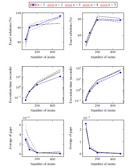Figure 1: MMACS with various values of α. Plots on the left show results for SCKP instances with a range of coefficients equal to 1000 and plots on the right show results for SCKP instances with a range of coefficients equal to 10000.

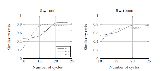Figure 2: Influence of α on the similarity of solutions found by MMACS algorithm for SCKP instances with 100 items.

Table 7: Percentage of exact solutions found by MMACS. The heuristic information value is fixed to β1 and the value of ρ varies between 0.01 and 1.

N	R			β1
		ρ1	ρ2	ρ3	ρ4	ρ5	ρ6
50	1000	82.0%	81.0%	83.0%	84.0%	83.0%	84.0%
	10000	55.0%	54.0%	48.0%	55.0%	50.0%	57.0%
100	1000	91.0%	86.0%	90.0%	87.0%	88.0%	87.0%
	10000	53.0%	51.0%	57.0%	53.0%	54.0%	55.0%
200	1000	84.0%	84.0%	82.0%	82.0%	84.0%	81.0%
	10000	55.0%	49.0%	46.0%	52.0%	53.0%	51.0%
500	1000	35.0%	40.0%	41.0%	37.0%	37.0%	34.0%
	10000	24.0%	28.0%	23.0%	27.0%	22.0%	27.0%

Table 8: Averages of solutions found by MMACS. The heuristic information value is fixed to β1 and the value of ρ varies between 0.01 and 1.

N	R			β1
		ρ1	ρ2	ρ3	ρ4	ρ5	ρ6
50	1000	0.08984	0.02556	0.03288	0.03032	0.03363	0.03963
	10000	0.02220	0.02653	0.01738	0.02172	0.01726	0.01966
100	1000	0.02126	0.01814	0.01206	0.02616	0.01718	0.04464
	10000	0.00870	0.00930	0.01639	0.00883	0.00897	0.01018
200	1000	0.00832	0.04333	0.02262	0.04705	0.00998	0.02377
	10000	0.00676	0.01265	0.00538	0.00577	0.01255	0.01741
500	1000	0.00676	0.16979	0.15236	0.11632	0.15827	0.17096
	10000	0.11085	0.12811	0.13676	0.12798	0.11106	0.12794

Table 9: Execution time of MMACS. The heuristic information value is fixed to 1 and the value of between 0.01 and 1.

N	R			β1
		ρ1	ρ2	ρ3	ρ4	ρ5	ρ6
50	1000	0.05492	0.05765	0.06821	0.05596	0.05465	0.05635
	10000	0.05567	0.05591	0.05756	0.05331	0.05382	0.05712
100	1000	0.39064	0.38973	0.76695	0.38287	0.39028	0.39951
	10000	0.38998	0.38882	0.77140	0.38358	0.39128	0.39009
200	1000	2.98575	3.00137	2.94311	2.93495	2.91098	2.95657
	10000	3.00461	2.95496	2.93763	2.91634	2.91860	2.95932
500	1000	48.0960	47.6133	46.3170	54.1633	46.7279	47.2380
	10000	47.9146	46.8829	46.5491	46.5299	46.7395	47.3001

N	R			β2
		ρ1	ρ2	ρ3	ρ4	ρ5	ρ6
50	1000	0.03299	0.03350	0.03077	0.05647	0.05426	0.03865
	10000	0.01685	0.01709	0.01783	0.01535	0.02255	0.02233
100	1000	0.01535	0.02211	0.01249	0.01724	0.01435	0.01480
	10000	0.00785	0.00968	0.01008	0.00698	0.00798	0.01020
200	1000	0.00337	0.00443	0.00610	0.00417	0.00520	0.00423
	10000	0.00116	0.00208	0.00217	0.00180	0.00181	0.00275
500	1000	0.06840	0.08212	0.06738	0.06309	0.07076	0.06730
	10000	0.03134	0.05077	0.03474	0.03055	0.03297	0.02785

Table 10: Percentage of exact solutions found by MMACS. The heuristic information value is fixed to β2 and the value of ρ varies between 0.01 and 1.

N	R			β2
		ρ1	ρ2	ρ3	ρ4	ρ5	ρ6
50	1000	80.0%	84.0%	82.0%	81.0%	84.0%	82.0%
	10000	52.0%	47.0%	51.0%	55.0%	54.0%	52.0%
100	1000	91.0%	93.0%	91.0%	90.0%	90.0%	91.0%
	10000	59.0%	59.0%	66.0%	60.0%	60.0%	55.0%
200	1000	86.0%	92.0%	90.0%	89.0%	90.0%	93.0%
	10000	62.0%	67.0%	68.0%	69.0%	65.0%	65.0%
500	1000	60.0%	63.0%	52.0%	58.0%	44.0%	59.0%
	10000	41.0%	37.0%	36.0%	36.0%	36.0%	33.0%

Table 11: Averages of solutions found by MMACS. The heuristic information value is fixed to β2 and the value of ρ varies between 0.01 and 1.

Table 12: Execution time of MMACS. The heuristic information value is fixed to  2 and the value of between 0.01 and 1.

N	R			β2
		ρ1	ρ2	ρ3	ρ4	ρ5	ρ6
50	1000	0.05313	0.05536	0.05604	0.05722	0.05452	0.05769
	10000	0.05358	0.05588	0.05365	0.05522	0.05618	0.05340
100	1000	0.37927	0.39185	0.38238	0.38306	0.38370	0.38917
	10000	0.38958	0.38976	0.39358	0.38518	0.38692	0.38878
200	1000	2.91574	2.96851	2.92166	2.91118	2.96750	2.97729
	10000	2.93331	2.91021	2.91412	2.95463	2.92098	2.94065
500	1000	46.3217	68.3414	46.0147	48.9379	47.6850	48.1014
	10000	46.0396	45.7421	46.2623	48.0479	46.4917	54.1009

N	R			β3
		ρ1	ρ2	ρ3	ρ4	ρ5	ρ6
50	1000	0.02858	0.03836	0.03311	0.03606	0.05618	0.03919
	10000	0.02232	0.02145	0.02609	0.02073	0.02204	0.02508
100	1000	0.02088	0.01689	0.01302	0.01218	0.01536	0.02067
	10000	0.00652	0.00897	0.00696	0.00931	0.00977	0.01037
200	1000	0.00353	0.00350	0.00293	0.00233	0.00261	0.00330
	10000	0.00093	0.00095	0.00117	0.00118	0.00161	0.00128
500	1000	0.02795	0.05289	0.04132	0.03866	0.03520	0.03838
	10000	0.01185	0.01029	0.01414	0.01199	0.00983	0.00629

Table 13: Percentage of exact solutions found by MMACS. The heuristic information value is fixed to β3 and the value of ρ varies between 0.01 and 1.

N	R			β3
		ρ1	ρ2	ρ3	ρ4	ρ5	ρ6
50	1000	81.0%	84.0%	83.0%	83.0%	79.0%	85.0%
	10000	50.0%	48.0%	49.0%	50.0%	54.0%	53.0%
100	1000	95.0%	89.0%	89.0%	91.0%	90.0%	94.0%
	10000	59.0%	63.0%	62.0%	61.0%	56.0%	57.0%
200	1000	92.0%	89.0%	93.0%	94.0%	92.0%	93.0%
	10000	72.0%	80.0%	77.0%	72.0%	73.0%	74.0%
500	1000	84.0%	88.0%	85.0%	84.0%	80.0%	86.0%
	10000	52.0%	50.0%	53.0%	46.0%	46.0%	49.0%

Table 14: Averages of solutions found by MMACS. The heuristic information value is fixed to β3 and the value of ρ varies between 0.01 and 1.

Table 15: Execution time of MMACS. The heuristic information value is fixed to  3 and the value of between 0.01 and 1.

N	R			β3
		ρ1	ρ2	ρ3	ρ4	ρ5	ρ6
50	1000	0.07581	0.07366	0.07465	0.07367	0.07425	0.07242
	10000	0.07422	0.07476	0.07528	0.07497	0.08080	0.07237
100	1000	0.46370	0.46119	0.46399	0.46445	0.45845	0.45893
	10000	0.46346	0.45978	0.46745	0.46602	0.46544	0.46089
200	1000	3.27010	3.26748	3.29506	3.30715	3.28653	3.24697
	10000	3.26838	3.27883	3.28464	3.30160	3.27514	3.24717
500	1000	50.0693	49.6441	49.2067	48.8005	48.5047	48.1483
	10000	49.8877	48.5299	48.9702	51.1495	48.8320	48.0786

N	R			β4
		ρ1	ρ2	ρ3	ρ4	ρ5	ρ6
50	1000	0.03218	0.03467	0.03252	0.03324	0.03187	0.03196
	10000	0.01684	0.02137	0.02540	0.02021	0.02979	0.02631
100	1000	0.01555	0.02284	0.01867	0.02045	0.02287	0.01441
	10000	0.00541	0.01040	0.00831	0.00895	0.00965	0.00892
200	1000	0.00263	0.00192	0.00176	0.00350	0.00185	0.00218
	10000	0.00104	0.00155	0.00142	0.00118	0.00127	0.00097
500	1000	0.02596	0.02232	0.03127	0.01763	0.01168	0.01989
	10000	0.00606	0.00439	0.00595	0.01001	0.00683	0.01049

Table 16: Percentage of exact solutions found by MMACS. The heuristic information value is fixed to β4 and the value of ρ varies between 0.01 and 1.

N	R			β4
		ρ1	ρ2	ρ3	ρ4	ρ5	ρ6
50	1000	84.0%	84.0%	82.0%	81.0%	80.0%	84.0%
	10000	51.0%	54.0%	51.0%	51.0%	51.0%	55.0%
100	1000	89.0%	90.0%	91.0%	91.0%	90.0%	93.0%
	10000	59.0%	61.0%	62.0%	67.0%	60.0%	53.0%
200	1000	91.0%	93.0%	92.0%	93.0%	91.0%	94.0%
	10000	83.0%	80.0%	81.0%	83.0%	78.0%	85.0%
500	1000	90.0%	93.0%	92.0%	89.0%	94.0%	85.0%
	10000	70.0%	70.0%	77.0%	65.0%	71.0%	74.0%

Table 18: Execution time of MMACS. The heuristic information value is fixed to  4 and the value of between 0.01 and 1.

N	R			β4
		ρ1	ρ2	ρ3	ρ4	ρ5	ρ6
50	1000	0.07929	0.08029	0.07424	0.07557	0.10963	0.07293
	10000	0.07846	0.07948	0.07611	0.07561	0.11752	0.07161
100	1000	0.49581	0.48432	0.48316	0.48317	0.48473	0.45665
	10000	0.49517	0.47001	0.49464	0.48414	0.48985	0.45644
200	1000	3.38250	3.28004	3.46215	3.45131	3.09758	3.22518
	10000	3.51687	3.29262	3.30075	3.45131	3.46598	3.23389
500	1000	48.3098	48.9813	47.9923	47.9734	49.1355	47.8999
	10000	48.7001	48.5943	48.7463	48.2574	48.2564	47.7792

N	R			β5
		ρ1	ρ2	ρ3	ρ4	ρ5	ρ6
50	1000	0.03247	0.03550	0.04044	0.06754	0.03757	0.03616
	10000	0.01910	0.03156	0.01838	0.01617	0.02353	0.02000
100	1000	0.01684	0.01483	0.01291	0.01588	0.01642	0.01395
	10000	0.00378	0.00786	0.00950	0.00682	0.00966	0.00802
200	1000	0.00218	0.00241	0.00284	0.00188	0.00210	0.00213
	10000	0.00129	0.00101	0.00097	0.00116	0.00158	0.00061
500	1000	0.00058	0.00188	0.00050	0.00265	0.00097	0.00283
	10000	0.00073	0.00460	0.00055	0.00069	0.00033	0.00348

Table 19: Percentage of exact solutions found by MMACS. The heuristic information value is fixed to β5 and the value of ρ varies between 0.01 and 1.

N	R			β5
		ρ1	ρ2	ρ3	ρ4	ρ5	ρ6
50	1000	82.0%	81.0%	81.0%	83.0%	79.0%	82.0%
	10000	49.0%	50.0%	47.0%	51.0%	44.0%	51.0%
100	1000	89.0%	91.0%	89.0%	88.0%	90.0%	89.0%
	10000	55.0%	58.0%	61.0%	55.0%	53.0%	59.0%
200	1000	91.0%	92.0%	90.0%	93.0%	92.0%	91.0%
	10000	79.0%	76.0%	81.0%	79.0%	76.0%	81.0%
500	1000	97.0%	98.0%	96.0%	95.0%	98.0%	97.0%
	10000	80.0%	78.0%	79.0%	79.0%	81.0%	77.0%

Table 21: Execution time of MMACS. The heuristic information value is fixed to β5 and the value of ρ varies between 0.01 and 1.

N	R			β5
		ρ1	ρ2	ρ3	ρ4	ρ5	ρ6
50	1000	0.07230	0.06982	0.07270	0.07362	0.07413	0.07302
	10000	0.07589	0.06936	0.07335	0.07472	0.07412	0.07157
100	1000	0.46598	0.47126	0.43751	0.46137	0.45676	0.45724
	10000	0.47470	0.46507	0.46672	0.46696	0.45895	0.45802
200	1000	3.34288	3.31321	3.31792	3.29320	3.27194	3.24836
	10000	3.09774	3.33303	3.35658	3.33049	3.28618	3.23154
500	1000	53.2248	48.9947	49.9506	48.2442	45.1045	44.6440
	10000	48.7456	49.1683	49.5907	49.3678	45.7457	48.2131

Table 22: Percentage of exact solutions found by MMACS. The values of q₀ are 0, 0.5, 0.75, 0.9 and 0.99.

N	R	q1	q2	q3	q4	q5
50	1000	83.0%	93.0%	84.0%	82.0%	66.0%
	10000	46.0%	61.0%	53.0%	52.0%	39.0%
100	1000	50.0%	86.0%	94.0%	90.0%	77.0%
	10000	11.0%	53.0%	67.0%	63.0%	36.0%
200	1000	15.0%	59.0%	88.0%	92.0%	88.0%
	10000	05.0%	23.0%	70.0%	79.0%	62.0%
500	1000	02.0%	12.0%	56.0%	98.0%	97.0%
	10000	01.0%	06.0%	24.0%	79.0%	85.0%

Table 23: Percentage of perfect solutions found by MMACS. The values of q₀ are 0, 0.5, 0.75, 0.9 and 0.99.

N	R	q1	q2	q3	q4	q5
50	1000	52.0%	62.0%	54.0%	52.0%	39.0%
	10000	12.0%	19.0%	16.0%	13.0%	6.0%
100	1000	44.0%	80.0%	87.0%	82.0%	68.0%
	10000	06.0%	36.0%	49.0%	46.0%	22.0%
200	1000	13.0%	56.0%	85.0%	88.0%	82.0%
	10000	05.0%	22.0%	66.0%	72.0%	56.0%
500	1000	01.0%	11.0%	55.0%	96.0%	95.0%
	10000	01.0%	06.0%	24.0%	78.0%	84.0%

Table 24: Averages of solutions found by MMACS. The values of q₀ are 0, 0.5, 0.75, 0.9 and 0.99.

	N	R	q1		q2		q3			q4	q5
	50	1000	0.02926		0.04270		0.07026			0.02934	0.31059
		10000	0.02430		0.01672		0.01380			0.02485	0.02395
	100	1000	0.08169		0.03278		0.01605			0.00887	0.01448
		10000	0.04577		0.00236		0.00286			0.00450	0.00636
	200	1000	0.16829		0.08070		0.00426			0.00248	0.00327
		10000	0.15506		0.03231		0.00146			0.00087	0.00090
	500	1000	0.33937		0.13807		0.06764			0.00059	0.00447
		10000	0.29663		0.12393		0.13807			0.00020	0.00026
ρ = 0.01				ρ = 0.02		ρ = 0.4			ρ = 0.5		ρ = 0.8		ρ = 1

200              400 Number of items

200              400 Number of items

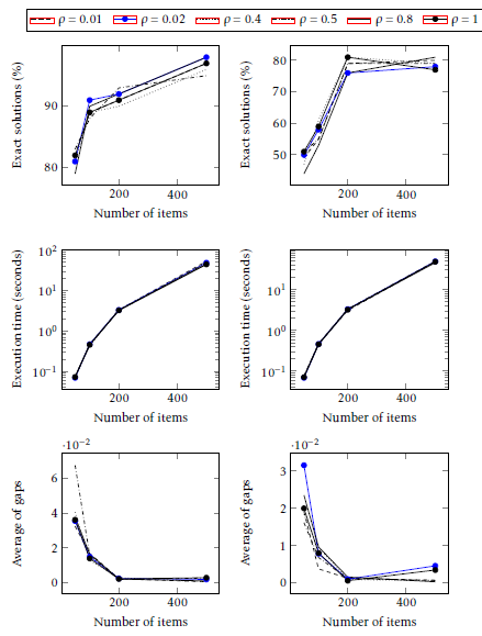Figure 3: MMACS with a fixed heuristic parameter β5 and various values of ρ . Plots on the left show results for

SCKP instances with a range of coefficients equal to 1000 and plots on the right show results for SCKP instances with a range of coefficients equal to 10000.

Table 25: Execution time of MMACS. The values of q₀ are 0, 0.5, 0.75, 0.9 and 0.99.

N		R	q1		q2		q3	q4		q5
50		1000	0.11231		0.06590		0.07087	0.05370		0.17519
		10000	0.14675		0.13272		0.24615	0.11360		0.15682
100		1000	1.11215		0.45967		0.59802	0.36749		1.04415
		10000	1.40685		1.06039		1.16371	0.73181		2.03097
200		1000	11.0831		7.03010		6.07585	1.64040		4.58164
		10000	11.3605		9.8870		11.0704	4.02055		11.2200
500		1000	189.264		162.474		114.984	10.5397		14.0793
		10000	179.640		175.398		162.474	38.1680		47.3076
	q = 0			q = 0.5		q = 0.75			q = 0.9		q = 0.99

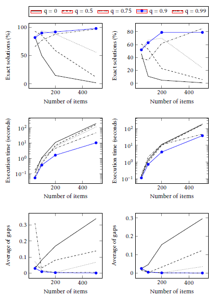Figure 4: MMACS with various values of q₀. Plots on the left show results for SCKP instances with a range of coefficients equal to 1000 and plots on the right show results for SCKP instances with a range of coefficients equal to 10000.

Table 26: Percentage of exact solutions found by MMACS. The number of ants varies between 1 and 100.

N	R	m1	m2	m3	m4	m5	m6
50	1000	41.0%	67.0%	77.0%	82.0%	86.0%	89.0%
	10000	25.0%	39.0%	45.0%	52.0%	59.0%	66.0%
100	1000	56.0%	84.0%	84.0%	90.0%	95.0%	93.0%
	10000	20.0%	42.0%	48.0%	63.0%	73.0%	84.0%
200	1000	72.0%	88.0%	90.0%	92.0%	94.0%	93.0%
	10000	18.0%	52.0%	67.0%	79.0%	89.0%	89.0%
500	1000	68.0%	86.0%	93.0%	98.0%	98.0%	98.0%
	10000	19.0%	53.0%	72.0%	79.0%	87.0%	90.0%

Table 27: Percentage of perfect solutions found by MMACS. The number of ants varies between 1 and 100.

N	R	m1	m2	m3	m4	m5	m6
50	1000	18.0%	40.0%	48.0%	52.0%	57.0%	59.0%
	10000	2.0%	5.0%	10.0%	13.0%	20.0%	24.0%
100	1000	48.0%	75.0%	77.0%	82.0%	87.0%	86.0%
	10000	7.0%	29.0%	29.0%	46.0%	54.0%	62.0%
200	1000	63.0%	83.0%	85.0%	88.0%	88.0%	88.0%
	10000	13.0%	47.0%	62.0%	72.0%	82.0%	81.0%
500	1000	66.0%	84.0%	90.0%	96.0%	97.0%	97.0%
	10000	16.0%	52.0%	71.0%	78.0%	86.0%	89.0%

Table 28: Averages of solutions found by MMACS. The number of ants varies between 1 and 100.

N	R	m1	m2	m3	m4	m5	m6
50	1000	0.17092	0.04399	0.05144	0.02934	0.03614	0.04252
	10000	0.06369	0.02088	0.02278	0.02485	0.01487	0.02389
100	1000	0.19670	0.02178	0.01721	0.00887	0.01573	0.01388
	10000	0.00962	0.01011	0.00449	0.00450	0.00639	0.00295
200	1000	0.01496	0.00345	0.00237	0.00248	0.00221	0.00198
	10000	0.00847	0.00139	0.00126	0.00087	0.00110	0.00127
500	1000	0.05480	0.01032	0.01423	0.00059	0.00679	0.00511
	10000	0.01608	0.00523	0.00092	0.00020	0.00028	0.00027

Table 29: Execution time of MMACS. The number of ants varies between 1 and 100.

N	R	m1	m2	m3	m4	m5	m6
50	1000	0.01501	0.03193	0.04690	0.05370	0.13695	0.23765
	10000	0.01918	0.04428	0.10274	0.11360	0.29489	0.53658
100	1000	0.06359	0.16153	0.35330	0.36749	0.60109	1.06442
	10000	0.07816	0.27944	0.50458	0.73181	1.55836	2.23375
200	1000	0.35064	0.81911	1.22310	1.64040	4.42083	8.29943
	10000	0.55900	2.20860	5.59126	4.02055	6.85303	10.5081
500	1000	5.07768	20.2446	20.4123	10.5397	34.7523	65.2062
	10000	8.64695	28.3465	44.5976	38.1680	118.269	153.611

Table 30: Number of problems solved by MMACS, MMAS, MMAS with 2opt, ACS, ACS with 2opt and QEA, in percentage

N	R	MMACS			MMAS		MMAS-2OPT			ACS			ACS-2OPT			QEA
		BS		PS	BS	PS	BS		PS	BS		PS	BS	PS		BS		PS
50	1000	82.0%		52.0%	75.0%	48.0%	77.0%		47.0%	49.0%		28.0%	60.0%	33.0%		0.0%		0.0%
	10000	52.0%		13.0%	41.0%	5.0%	44.0%		5.0%	31.0%		4.0%	34.0%	5.0%		0.0%		0.0%
100	1000	90.0%		82.0%	38.0%	36.0%	45.0%		40.0%	63.0%		60.0%	69.0%	0.0%		0.0%		0.0%
	10000	63.0%		46.0%	10.0%	5.0%	14.0%		5.0%	28.0%		15.0%	22.0%	9.0%		0.0%		0.0%
200	1000	92.0%		88.0%	12.0%	12.0%	16.0%		13.0%	75.0%		73.0%	74.0%	70.0%		0.0%		0.0%
	10000	79.0%		72.0%	2.0%	2.0%	3.0%		3.0%	36.0%		32.0%	26.0%	21.0%		0.0%		0.0%
500	1000	98.0%		96.0%	2.0%	2.0%	3.0%		1.0%	65.0%		65.0%	69.0%	66.0%		0.0%		0.0%
	10000	79.0%		78.0%	0.0%	0.0%	1.0%		0.0%	29.0%		28.0%	34.0%	33.0%		0.0%		0.0%
1000	1000	100%		96.0%	0.0%	0.0%	2.0%		1.0%	38.0%		38.0%	40.0%	40.0%		0.0%		0.0%
	10000	90.0%		90.0%	0.0%	0.0%	2.0%		2.0%	20.0%		20.0%	20.0%	20.0%		0.0%		0.0%
2000	1000	100%		98.0%	0.0%	0.0%	1.0%		1.0%	40.0%		40.0%	10.0%	10.0%		0.0%		0.0%
	10000	96.0%		94.0%	0.0%	0.0%	0.0%		0.0%	30.0%		30.0%	0.0%	0.0%		0.0%		0.0%
			m = 1        m = 5					m = 10        m = 20			m = 50				m = 100

200              400 Number of items

200              400 Number of items

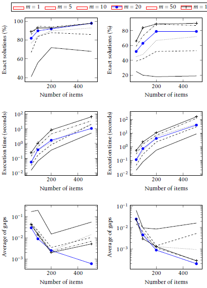Figure 5: MMACS with various values of the number of ants. Plots on the left show results for SCKP instances with a range of coefficients equal to 1000 and plots on the right show results for SCKP instances with a range of coefficients equal to 10000.

Table 31: Average of GAPS of MMACS, MMAS, MMAS with 2opt, ACS, ACS with 2opt and QEA

N	R	MMACS	MMAS	MMAS-2OPT	ACS	ACS-2OPT	QEA
50	1000	0.02934	0.23080	0.02355	0.35243	0.02780	15.9902
	10000	0.02485	0.09708	0.02444	0.29466	0.03918	19.0041
100	1000	0.00887	0.76940	0.08039	0.13530	0.01213	39.4817
	10000	0.00450	0.50409	0.04409	0.08419	0.00915	39.6268
200	1000	0.00248	0.16937	0.16207	0.20180	0.02418	55.7324
	10000	0.00087	0.15295	0.14329	0.03192	0.00513	50.7264
500	1000	0.00059	0.33796	0.33374	0.04334	0.04135	92.6842
	10000	0.00020	0.30745	0.30680	0.02888	0.02113	91.554
1000	1000	0.00000	0.79903	0.42312	0.04723	0.09261	109.042
	10000	0.00015	0.83977	0.43098	0.10385	0.15489	115.452
2000	1000	0.00000	1.27071	0.49220	0.10819	0.09249	123.848
	10000	0.00001	1.33153	1.37336	0.08955	0.16696	130.323

Table 32: Execution time of MMACS, MMAS, MMAS with 2opt, ACS, ACS with 2opt and QEA, in seconds

N	R	MMACS		MMAS	MMAS-2OPT		ACS	ACS-2OPT		QEA
50	1000	0.05370		0.10212	0.10072		0.11601	0.11575		0.73706
	10000	0.11360		0.25768	0.15341		0.15797	0.14653		0.70629
100	1000	0.36749		1.72373	1.06384		0.68345	0.55707		2.30542
	10000	0.73181		1.37522	1.38279		1.10934	1.06852		2.31311
200	1000	1.64040		19.1191	9.92326		3.65467	3.44395		8.40170
	10000	4.02055		11.0615	10.2807		7.45693	8.76620		8.21929
500	1000	10.5397		189.923	182.438		67.8814	61.3986		46.9157
	10000	38.1618		195.993	164.348		131.969	127.623		46.3203
1000	1000	47.9736		829.651	1284.21		898.149	326.323		174.192
	10000	191.046		867.371	1281.49		730.028	420.990		183.470
2000	1000	340.109		3332.80	1437.79		3648.84	4474.66		722.961
	10000	1318.38		3359.86	3152.59		4253.97	4566.97		781.133
			MMACS			MMAS-2opt          ACS-2opt

0

1,000              2,000 Number of items

0

1,000              2,000 Number of items

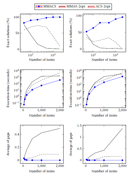Figure 6: Comparison of MMACS, MMAS with 2-opt and ACS with 2-opt results. Plots on the left show results for SCKP instances with a range of coefficients equal to 1000 and plots on the right show results for SCKP instances with a range of coefficients equal to 10000.

reduce the time. The values 20, 50 and 100 give almost the same percentages. Thus, the value 20 gives the best compromise between a reasonable execution time and acceptable solutions. The solutions are satisfying regarding the considerable percentage of exact solutions and the reduced gap values.

6.3. MMACS experimental settings

We have fixed the parameter values after a set of experimental tests. We have set α to 1, β to 5 and ρ to 0.02, where α and β are the two parameters that determine the relative importance of the pheromone and the heuristic factors and ρ is the evaporation factor. The number of cycles were set to 20 and 20 is the number of ants. As for pheromone trails bounds, we have set τ_max to 6 and τ_min to 0.01. Finally, the fixed parameter q₀ was set to 0.9.

6.4. MMACS results

After fixing the parameter values of MMACS, empirical results are presented in this section. At a first stage, MMACS results are compared with those of MMAS [9, 10] and ACS [11]. After that, the performances of MMACS while solving SCKP are evaluated and compared to recent methods in the literature: the 2-optimal heuristic [5] and the QEA algorithm [6].

6.4.1. Comparison of MMACS, MMAS and ACS

We test MMACS and the two ACO algorithms: MMAS [9, 10] and ACS [11]. Then, we compare the obtained results. Table 1 gives the default values of the ACO parameters. MMACS, MMAS and ACS were performed on Pisinger instances of size 50, 100, 200, 500, 1000 and 2000. MMAS and ACS were tested with and without the employment of a local search. Results are given in Tables 30- 32. Their performance was compared in terms of percentage of exact and perfect solutions in Table 30, deviation of the best solution found from the optimal solution in Table 31 and the execution time in Table 32. Then, the three ACO algorithms are compared in Figure 6. Results show that for all instances, MMACS algorithm outperform the two ACO algorithms in terms of percentage of exact solutions, execution time and deviation of the best solution found from the optimal solution.

6.4.2. Comparison of MMACS with state of art algorithms

Experiments were conducted on two sets of instances and presented in this section. In the first part of experiments, MMACS, 2-optimal heuristic and QEA solve the instances of the Pisinger set. In the second part, MMACS an QEA were used to solve the instances of the generated set.

Experimental results on the instances of the Pisinger set: We present in this part the results of the experiments realized on the Pisinger set instances of the Strongly Correlated Knapsack Problems. Table 33 shows that in most cases, MMACS turned out to outperform both state of art algorithms. In fact, QEA could not solve these problems to optimality, unlike 2-optimal heuristic which showed better results than MMACS in one case out of four. Besides, our proposed algorithm MMACS reached one hundred percent of solved problem starting with the number of items equal to 1000 and a range of coefficients equal to 1000.

Table 33: Percentage of problems solved by 2–optimal heuristic, MMACS algorithm and QEA algorithm

N	R	2-Optimal	QEA	MMACS
100	1000	68.9%	0%	90%
	10000	13.9%	0%	63%
1000	1000	99.6%	0%	100%
	10000	96.7%	0%	90%
2000	1000	100%	0%	100%
	10000	100%	0%	100%

Experimental results on the instances of the generated set: Additional experiments were conducted on the instances of the generated set. We compare the results of the MMACS algorithm with a state of art algorithm QEA [6]. In QEA, the population size, the maximum number of generations, the global migration period in generation, the local group size and the rotation angle were set to 10, 1000, 100, 2 and 0.01 π, respectively.

Both algorithms MMACS and QEA were run under the same computational conditions on instances of the generated set.

In experiments of this part, the SCKP numeric parameters were set to the following values: R = 10, k = 5 and the number of items are 100, 250 and 500. The generated instances used here are similar to those presented in [6].

The exact solutions of generated instances were obtained using a dynamic programming algorithm [16] that we implemented.

Table 34 shows that MMACS found 30/30 exact solutions for all instances where MMACS BFS (best found solutions) are equal to the optima. Those significant results were given within an acceptable execution time when compared with QEA. The execution time (CPU) and the gap between the found solution and the optimum (Gap) were averaged over 30 runs.

Besides, MMACS and QEA were compared using Wilcoxon Signed Rank Test [17]. This nonparametric test shows that the two groups of data are different according to z-statistic value and p-value at the 0.01 significance level, as shown in Table 35.

Table 34: Comparative results of MMACS algorithm with a state of art algorithm QEA

N		QEA				MMACS
	BFS	Gap	CPU	BS	BFS	Gap	CPU	BS
100	572	7.43099	1.04186	0%	607	0.00	0.00423	100%
250	1407	11.7935	4.48270	0%	1547	0.00	0.05806	100%
500	2115	20.5593	15.5481	0%	2499	0.00	0.98446	100%

Table 35: Comparative results of MMACS and QEA using Wilcoxon Signed Rank Test

N	z-satistic	p-value
100	-4.7821	0.00000
250	-4.7821	0.00000
500	-4.7821	0.00000

7. Conclusion

The paper presents a comparative study of the proposed hybrid algorithm MMACS while solving the strongly correlated knapsack problems. We gave an experimental analysis of the impact of different parameters on the behavior of MMACS algorithm. Experiments show that the default parameter settings proposed in the literature, gave the best possible results essentially in terms of execution time. It is also noticed from the results that ants in MMACS construct solutions relying mainly on the heuristic information rather than pheromone trails. In fact, initializing pheromone trails to the upper bound helps ants to start the search in promising zones. Besides, the MMACS balances between exploitation and exploration by the employment of a choice rule that alternate between greedy and stochastic approaches. Then, MMACS results were compared to those of MMAS and ACS, the three algorithms show very different behaviors when solving SCKP. The MMACS algorithm outperforms both ant algorithms. In the second part of experiments, we compared MMACS to other recent metaheuristics. Basically, MMACS gave better quality of solutions. As perspective, we propose to draw more attention to the exploitation of the best solutions, in order to avoid early search stagnation. This can achieve the best performances of MMACS.

Conflict of Interest

The authors declare no conflict of interest.

1.  W. Zouari, I. Alaya, M. Tagina, “A hybrid ant colony algorithm with a local search for the strongly correlated knapsack problem” in 2017 IEEE/ACS 14th International Conference on Computer Systems and Applications (AICCSA), Hammamet Tunisia, 2017. https://doi.org/10.1109/aiccsa.2017.61
2.  D. Pisinger, “Core problems in knapsack algorithms” Oper. Res., 47 (4), 570–575, 1999. https://doi.org/10.1287/opre.47.4.570
3.  T. Cormen, C. Leiserson, R. Rivest, C. Stein, “Greedy algorithms” Introduction to algorithms, 1990. https://doi.org/10.2307/2583667
4.  St ¨ utzle, Thomas and Ruiz, Rub´en, Iterated greedy, Handbook of Heuristics, Springer, 2018. https : ==doi:org=10:1007=978-3-319-07124-410
5.  D. Pisinger, “A fast algorithm for strongly correlated knapsack problems” Discrete Appl. Math., 89 (1-3), 197–212, 1998. https://doi.org/10.1016/s0166-218x(98)00127-9
6.  K.-H. Han, J.-H. Kim, “Quantum-inspired evolutionary algorithm for a class of combinatorial optimization” IEEE Trans. Evol. Comput., 6 (6), 580–593, 2002. https://doi.org/10.1109/tevc.2002.804320
7.  K. O. Jones, “Ant colony optimization, by marco dorgio and thomas st ¨ utzle” ROBOTICA, 2005. https://doi.org/10.1017/s0269888905220386
8.  Dorigo, Marco and St ¨ utzle, Thomas, Ant colony optimization: overview and recent advances, Handbook of metaheuristics, Springer, 2019. https : ==doi:org=10:1007=978-3-319-91086-410
9.  T. St ¨ utzle, H. Hoos, “Max-min ant system and local search for the traveling salesman problem” in IEEE International Conference on Evolutionary Computation, Indianapolis USA, 1997. https://doi.org/10.1109/icec.1997.592327
10.  T. St ¨ utzle, H. H. Hoos, “Max–min ant system” Future Gener. Comput. Syst., 16 (8) 889–914, 2000. https://doi.org/10.1016/s0167-739x(00)00043-1
11.  M. Dorigo, L. M. Gambardella, “Ant colony system: a cooperative learning approach to the traveling salesman problem” IEEE Trans. Evol. Comput., 1 (1), 53–66, 1997. https://doi.org/10.1109/4235.585892
12.  I. Alaya, C. Solnon, K. Ghedira, “Ant colony optimization for multi-objective optimization problems” in 19th IEEE International Conference on Tools with Artificial Intelligence(ICTAI 2007), Patras Greece, 2007. https://doi.org/10.1109/ictai.2007.108
13.  G. A. Croes, “A method for solving travelingsalesman problems” Oper. Res., 6 (6), 791–812, 1958. https://doi.org/10.1287/opre.6.6.791
14.  T. St ¨ utzle, M. L´opez-Ib´anez, P. Pellegrini, M. Maur, M. M. De Oca, M. Birattari, M. Dorigo, Parameter adaptation in ant colony optimization, Autonomous search, Springer, 2011. https://doi.org/10.1007/978-3-642-21434-9 8
15.  R. W. Morrison, K. A. De Jong, “Measurement of population diversity” in International Conference on Artificial Evolution (Evolution Artificielle), Berlin Heidelberg, 2001. https://doi.org/10.1007/3-540-46033-0 3
16.  P. Toth, “Dynamic programming algorithms for the zeroone knapsack problem” Computing, 25 (1), 29–45, 1980. https://doi.org/10.1007/bf02243880
17.  F. Wilcoxon, S. Katti, R. A. Wilcox, Critical values and probability levels for the wilcoxon rank sum test and the Wilcoxon signed rank test, Selected tables in mathematical statistics 1, 1970.

(Click Here)

(Click Here)