1. Introduction

This paper is an extension of work originally presented as well as choices concerning the number and configin 2017 IEEE 20th International Conference on Intelli- uration of the approach and exit lanes, priority hanging Transport Systems [1]. Where our previous work dling, slow traffic crossing facilities, signal control and was a first evaluation of using traditional decision tree geometric attributes such as the lane length and the algorithms in order to predict a set of (Pareto optimal) central reservation width. The need to determine the junction design alternatives, we now extended the ap- best junction design is not only triggered by the conproach, applied and evaluated it on cases for two differ- struction of new infrastructure. Due to changes in ent countries and compared the results with existing traffic volumes, travel routes and vehicle types there is junction design rules by comparing both accuracy and a regular need for re-evaluation of the junction design. performance.

The junction design assessment process, which is used to select the best alternative, typically involves three stages [2]. In the first stage, viable alternatives are identified based on limited input data, such as the average annual daily traffic volume, using decision rules, in the form of trees, look-up tables or simple calculation methods, provided in design manuals. In the second stage, more detailed input data, such as the peak hour traffic volumes for each turning movement and specific geometric and control attributes, are collected and the operational, safety and environmental performances are determined by using tools ranging from static analytical to dynamic simulation models. In the third stage, the best alternative is selected based on multiple criteria. The performance measures determined in the previous stage are analysed and weighted in combination with other criteria such as specific local constraints and cost, before selecting the best alternative. This three-stage approach is used to avoid time and money consuming assessment of many alternatives, but possesses the risk of omitting the best solution due to a deficient identification of viable alternatives in the first stage of the assessment process [3]. This deficiency is mostly caused by a lack of consciousness concerning which objectives are served by the rules used in this stage.

The availability and quality of the decision rules used to identify the viable alternatives varies by state, region or country. The rules have been developed over a period of many years based on a combination of data collection and expert judgement. Obviously, this is a positive feature, but also comprises some disadvantages. First, the decision rules do not offer a complete and consistent approach for all junction design alternatives. Some rules are only meant for signalised junctions where others only encompass whether a left-turn bay is needed on a major road approach to a priority junction. Some rules are formal warrants where others are informal guidelines. Second, many decision rules have not been updated for many years and thus do not reckon with changes in traffic behaviour and vehicle types and do not include relatively new junction design alternatives. Third, rules are often based on one underlying objective, generally referring to the operational performance, causing junction design alternatives that are better or best for other objectives to be neglected. Other rules implicitly contain a weighing or preferred order for different objectives, which restricts and complicates the assessment of multiple objectives in a later stage of the junction design assessment process.

Surprisingly, only limited efforts have been made to develop new junction design rules. [4] used the HCM 2010 methodologies [5] to distinguish between different junction types based on the major and minor street volumes. They generated a dataset with more than 6,000 scenarios of varying traffic flows for three main junction types. The results were plotted in 2- and 3D diagrams using the major an minor volumes and the average control delay classified by junction type, in order to identify the areas where a junction type has the lowest delay. [6] used the HCM 2000 methodologies [7] to determine so-called shape-grammars for junction type choice based on the total traffic volume and the through traffic share for three and four arm junctions resulting in look-up tables. Although these studies provided interesting approaches, they examine a limited number of junction designs and demand volumes and moreover, they conducted a manual analysis of the generated data. [8] generated a dataset with the operational performance of 1,296 scenarios for different junction design types and traffic patterns using VISSIM, determining the total delay, stop delay and the average number of stops per vehicle. A classification tree method was then used to group the scenarios into as many homogeneous classes as possible. Classes were constructed for capacity shortage as well as delay. Based on these classes one can easily discover the average operational performance for one or more junction design alternatives. Still, the resulting classes do not provide a set of viable junction design alternatives and are only based on the operational objective.

In this paper, we present an approach by which new junction design rules can be determined. The resulting rules can be used to predict a set of viable junction design alternatives for the first stage of the junction design assessment process. The predicted set is in fact the Pareto optimal set of solutions for multiple objectives, e.g. regarding operational, safety and/or environmental impact. The Pareto optimal set of solutions always contains the best solution, whatever set of weights is used for different objectives in a later stage of the assessment process, thus handling multiple objectives in a straightforward manner. The rules are derived from a dataset by using decision tree data mining techniques. For this, a large dataset is needed, which is first generated, using performance models, with Pareto optimal sets of junction design alternatives for a large amount of, randomly generated, traffic volumes. The approach is applied and evaluated on cases in two different countries.

In the next section, we will first explain the suggested approach. Subsequently, in section 3, the evaluation framework will be discussed. In section 4 the existing junction design rules and the implementation of the approach for the two cases will be explained. The results are discussed in section 5. The paper ends with conclusions in section 6.

2. Approach

In this section we will explain our approach for determining junction design rules used to select viable junction design alternatives based on multiple objectives. The approach consists of three major steps:

1. Define the scope
2. Generate the dataset
3. Determine the decision tree

In the first step, choices are made concerning the junction design alternatives, the traffic flow ranges and the objectives to be considered. In the second step, a dataset is generated containing a Pareto optimal set of junction design alternatives for each, randomly generated, traffic flow pattern. Each set is determined after running performance models for each objective and junction design alternative. In the third step, decision tree algorithms are used to derive rules from the dataset. The steps will be explained in more detail in the next paragraphs.

2.1.  Define the scope

In the first major step, choices are made concerning the:

• Junction designs
• Traffic flows
• Objectives
• Performance models

First, the junction design alternatives to be considered should be defined. This is a list of all the possible junction design alternatives that should be evaluated. Junction design involves both the choice for the main type, such as signalised junction or roundabout, as well as choices concerning the number and configuration of the approach and exit lanes, priority handling, slow traffic crossing facilities, signal control and geometric attributes such as the lane length and the central reservation width. The level of detail depends upon the requirements for the specific case. An important issue involves the necessity to classify the junction design alternatives by a size category. This attribute was introduced in order to prevent large (or expensive) junctions always to be the preferred design, regardless of the traffic flow volumes on the junction.

Second, it should be decided for which traffic flow ranges the junction design alternatives should be evaluated. The traffic flow at least involves the turning volumes for the motorised vehicles on the junction. Additionally, pedestrian and bicycle volumes can be used as well. Typically, peak hour volumes are used, since these are major input variables for the performance model(s) used. The range, i.e. the total traffic volume on the junction, is case specific and dependent upon the chosen junction design alternatives.

Third, it should be decided based on which objectives the junction design alternatives should be evaluated. Typically, minimising the operational performance, e.g. the average delay, is used. Additionally, safety, environmental and financial performance measures can be used. The choice is strongly influences by the possibilities to model the performance measures. The suggested approach assumes at least two objectives in order to determine Pareto optimal sets of junction design alternatives.

Fourth, in close connection with the other choices, it should be decided which performance model will be used. The model uses the traffic flows and junction design alternative as input. There is a wide range of models available to determine the performance for a specific objective, ranging from static analytical to dynamic simulation models. The choice depends upon the models and underlying methodologies that are accepted in a specific country, and/or the accepted level of detail of input data or the calculation time of the models. Separate models can be used for separate objectives.

In order to illustrate our approach, we will use a simplified example case. Table 1 shows six four-arm junction design alternatives, with four main junction types, being all-way stop controlled junction (AW), two-way stop controlled junction (TW), signalized junction (SIG) and roundabout (RA). Two size categories (Sc) are differentiated and the lane number and configuration for the approach and exit lanes of the major and minor roads are defined for each alternative. The lane configuration means that there is one lane which is shared by left turning, straight and right turning traffic, whereas means that there are two lanes; a separate lane for left turning traffic and a shared lane for straight and right turning traffic.

Table 1: Simplified example with the definition of six junction design alternatives

For the traffic flows, only motorized vehicles are used, where the total traffic flow on the junction is assumed to range between 0 and 2000 pcu/h. Two objectives, being operation and safety will be used, respectively expressed by the (volume weighted) average delay (s) and the estimated number of fatal injuries per year. A fictitious performance model is assumed to generate the measures for this example case. Additionally, a delay threshold of 50 seconds is used, in order to exclude junction design alternatives with an undesirable operational performance.

2.2. Generate the dataset

In the second major step, a dataset is generated that contains a set of junction design alternatives for each combination of traffic demand pattern and size category. This set of junction design alternatives for each combination is the Pareto optimal set of solutions for multiple objectives. The Pareto optimal set is determined by determining the performances for each junction design alternative given a (randomly generated) traffic demand pattern. The performances are determined by using a traffic performance model that uses the traffic demand pattern and junction design as input. It is necessary to generate the data by using performance models, since consistent and comprehensive data is not available from surveys.

Objective	Performance measure	Value
Operation	Average delay (s)	12.31
Safety	Fatal injuries per year	0.42

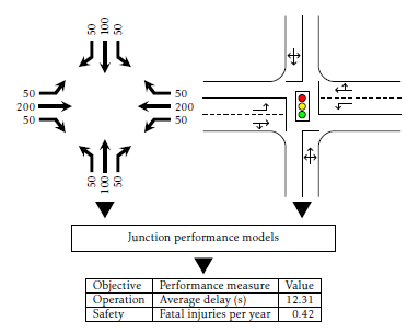Figure 1: Schematic representation of performance modelling for one specific traffic demand pattern and junction design alternative

Figure 1 shows a schematic representation of the performance modelling for one specific traffic demand pattern (with a total volume of 1000 pcu/h) and a junction design alternative (SIG2 from Table 1). This results in a (volume weighted) average delay of 12.31 seconds and an estimated number of fatal injuries of 0.42 per year. For the given traffic demand pattern, this is repeated for each junction design alternative that has been defined. The operational and safety performances of the six junction design alternatives are shown in Figure 2 for both size categories.

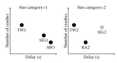Figure 2: Set of junction design alternative solutions for two different size categories

The main question now is, which junctions design alternatives should be part of the viable set of solutions? The best choice would be the Pareto optimal set of solutions. The Pareto set consists of all solutions for which the corresponding objective values cannot be improved for one objective, without degradation of the other. As said, the Pareto optimal set of solutions always contains the best solution, whatever set of weights are used for the operational or safety performance in a later stage of the assessment process. The Pareto optimal solutions can be determined automatically. In our example, for the first size category, the Pareto optimal solution would be {AW1,TW1,SIG1}.

For the second size category it would be {TW2,RA2}. Additionally, solutions with a performance above a certain threshold value, e.g. a specific average delay, could be removed from the viable solution set, in order to prevent analysis of unrealistic solutions in a later stage of the assessment process.

The described process is repeated for multiple (randomly generated) traffic demand patterns. The number of traffic demand patterns to be generated is case specific and should be determined based on the accuracy of the tree to be predicted in the next main step. The accuracy represents how well the tree predicts the Pareto optimal sets that are used as input. This will be explained in more detail in section 3. In earlier experiments [9] we tested the approach for 10thousand, 100-thousand and 1-million traffic demand patterns. Although, the predictive accuracy of the trees increased with bigger datasets, the differences between the set sizes were minimal. Table 2 shows an example dataset for only four traffic demand patterns. The dataset contains both the variables representing the base traffic pattern, i.e. the volumes for the twelve turning movements as shown in Figure 1 (v1-v12), as well as multiple combined variables such as the total volume on the major (vMa) or minor road (vMi) or the whole junction (vTot). The combined variables are important for the rules to be determined.

Table 2: Simplified example dataset with four traffic demand patterns

Id	v1	v2	…	v12	vMa	vMi	vTot	Sc	Set
1	25	100		25	300	200	500	1	{AW, TW}
2	25	100		25	300	200	500	2	{TW, RA}
3	50	200		50	600	400	1000	1	{AW, TW, SIG}
4	50	200		50	600	400	1000	2	{TW, RA}
5	75	300		75	900	600	1500	1	{SIG}
6	75	300		75	900	600	1500	2	{SIG, RA}
7	100	400		100	1200	800	2000	1	{OTHER}
8	100	400		100	1200	800	2000	2	{RA}

The table also shows a solution set {OTHER}. For this combination of traffic demand pattern and size category, there was no junction design alternative with a delay below the chosen threshold value (50 seconds). The set is included in the dataset in order to facilitate rules that advise an ’other’ solution for the specified combination of traffic demand pattern and size category. The created dataset is the foundation of the training set used to determine the decision tree (and the rules) in the next major step.

2.3. Determine the decision tree

In the third major step, the decision tree is determined. Decision trees use a white box model, are easy to understand and interpret, perform well on large datasets, are robust and offer possibilities to validate the model using statistical techniques [10]. Most important, rules can be read from the resulting trees. Determining a tree which can be used to predict a set of junction design alternatives is basically a multi-labelled decision tree challenge [11]. A modest number of algorithms have been suggested to construct multi-labelled decision trees [12, 13, 14, 15, 16, 17]. In these algorithms, various functions in the traditional decision tree algorithms are replaced by functions fit for handling multi-labelled data, primarily based on measures for the similarity between one or more sets. Unfortunately, these algorithms have some serious disadvantages, the most important one being the fact that they produce very large and complex trees, which is caused by their lack of pruning methods. To overcome these difficulties, we introduced an alternative approach [1]. In this approach we normalise the training data and use the predicted probabilities of the resulting tree, confronted with a threshold value, to determine multiple target labels. This enables us to predict sets of junction design alternatives with traditional algorithms and thus having the advantage of using profoundly proven and widely available methods with a range of modelling options, such as pruning. This approach consists of three (sub)steps:

• Normalise the data
• Built a decision tree
• Determine predicted sets of solutions

2.3.1.  Normalize the data

The first step is to apply the standard data normalization method [18], which is needed when using single labelled decision tree algorithms. This method transforms the data into single-labelled instances. The example training set from Table 2, would then be transformed to the data set with fourteen instances. One instance for each set element. An instance with a set of three junction design alternatives (id 1 in Table 2) is transformed to three instances with one junction design alternative.

2.3.2.  Built a decision tree

In the second step, traditional, single-labelled, decision tree algorithms such as ID3, C4.5, CRT, CHAID and QUEST can be used to build a tree. Most of these decision tree algorithms consist of two conceptual phases: growing and pruning. In the tree growing phase, a tree is constructed by using an iterative procedure, were in each iteration the algorithm considers the partition of the training set by selecting the most appropriate attribute according to some splitting measure(s). The tree growing phase continues until a certain stopping criterion is triggered, e.g. when all instances in nodes belong to one class or when a maximum tree depth has been reached. In the pruning phase, the size of the tree is reduced by removing sections of the tree that provide little power to classify the instances. Pruning reduces the complexity of the final tree and hence improves predictive accuracy by reduction of over-fitting.

A major point of criticism for single-labelled decision tree algorithms, is that the obtained classifier could only predict a single label [13]. However, this is only partly true. Although the decision tree algorithms aim to produce nodes and leaves which contain elements with the same label, leaves more often contain elements with multiple labels. This is particularly true for situations where all the instances in a node have (nearly)the same attributes, as a result of which no attribute and value can be determined to split the instances any further. In our example, the normalized instances coming from one set have the same attributes. When there is a sufficient amount of instances in a leaf, i.e. small tree and large dataset, a leaf contains a probability vector, were the probability is determined by comparing the frequency of the instances with a specific label with the total number of instances in the leaf. This probability vector in combination with the normalization method, offers the opportunity to use the single labelled methods for multiple labelled data.

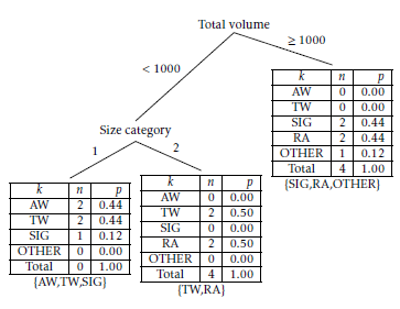Figure 3: Example decision tree with predicted probabilities

Figure 3 shows the decision tree based on our example training set, but now including the number of instances (count and percentage) for each junction design alternative (k) in each leaf. The percentage represents the predicted probability. Based on preliminary tests we concluded that the CRT decision tree algorithm performed best for our problem. CRT [19] performs binary splits based on a Gini impurity measure and allows pruning.

2.3.3. Determine predicted set of solutions

In the third step, the predicted set of junction design alternatives can be derived from the frequencies and/or predicted probabilities. In our case, a junction design alternative is included in the predicted set if the predicted probability in the leaf is greater than zero. For our example, the predicted set of junction design alternatives is shown at the bottom of each leaf, as can be seen in Figure 3. Alternative threshold values (τ) can be used to determine the predicted sets to reduce the number of junction design alternatives in the sets. Higher values of τ will produce smaller predicted sets of solutions, but with a higher change of missing junction design alternatives. Lower values of τ will produce larger predicted sets of solutions, but with a higher change of overestimating the number of viable junction design alternatives. The optimal value for τ is to be determined, but can be chosen after the decision tree has been built. Moreover, this variable can either be determined static (1) or dynamic (2):

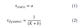Where K is the number of possibly predicted junction design alternatives in the regarding leaf and a and b are constants. In our case K, is dependent upon the size category, since not each size category has the same number of junction design alternatives. In our small example (Figure 3), size category 1 does not include the roundabout, so K would be 4, as can be seen in the leftmost leaf. For size category 2 K is equal to 5, as can be seen in the central leaf. If the size category is not a split attribute, or multiple size categories are combined in one leaf, the highest number for K is presumed, as is the case for the rightmost leaf. Based on preliminary tests we concluded that a dynamic determination of τ with d = 1 gave best results.

3. Evaluation framework

We will apply the approach on two cases. The cases will be explained in section 4. In order to determine the success of the approach for the two cases, the new rules resulting from the approach are compared with existing rules. First the predictive accuracy of the rules will be evaluated. This will give insight in how good the rules can reproduce the Pareto optimal set of solutions from the generated dataset as described in section 2.2. Secondly, the performances of the predicted sets of viable junction design alternatives will be evaluated. This will give insight in the average and/or minimal (e.g. operational, safety and environmental) performances of the junction design alternatives that are predicted by the rules. Two-third of the dataset, as described in section 2.2, is used to train the model for the new rules. One-third is used to evaluate both the new and existing rules. The latter is the test set.

3.1. Accuracy

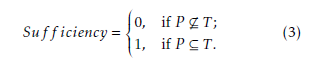
In situations with single-labelled data, the predictive accuracy of a rule is simply the proportion of correctly classified or predicted instances. If we would apply this to our multi-labelled data, this is a very strict measure, being the proportion of instances for which the predicted set of labels is the same as the true set of labels. In our context, predicting a set of viable junction design alternatives for further research, we are also interested in the proportion of instances for which the predicted set at least contains the true set of labels. In this context predicting too much labels instead of predicting too few is less bad. Therefore, we introduce using multiple measures to evaluate the accuracy of the rules. All accuracy measures discussed are on a per instance basis and the aggregate value is an average over all instances. Let T be the true set of labels (i.e. the Pareto optimal set) and P be the predicted set of labels (i.e. by either the new or existing rules). The measure for the predicted set at least containing the true set, we name sufficiency, which is defined as:

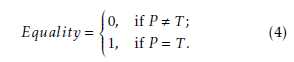
The measure for the predicted set being equal to the true set, we name equality, which is defined as:

Although predicting to much labels is less bad than predicting too few, it is still a disadvantage of the model. Therefore, we also evaluate the number of labels that is wrongfully predicted with the overestimation measure:

This measure is best evaluated in relation with the average set size.

Additionally, we use a similarity measure which is a more general measure for comparing sets used by various authors [13, 14, 17], also referred to as the Jaccard index or intersection over union:

The values for sufficiency, equality and similarity range between 0 and 1. Higher values correspond to higher accuracy. The value of overestimation ranges from 0 up to the maximum number of labels. Lower values correspond to higher accuracy.

In order to determine the strengths and weaknesses of the new rules, it is imperative to differentiate the indicators for different size and volume categories.

3.2. Performance

An important issue involves the fact that existing rules are often based on one objective, thereby neglecting junction design alternatives that are important for other objectives. If a rule selects viable junction design alternatives based on minimizing the average delay, the alternative with the lowest number of accidents could be missing from the predicted set. It is important to compare the performances resulting from the new and existing rules in relation to the performances resulting from the Pareto optimal set. Various indicators exist for this purpose. [20] provided an excellent overview in the context of comparing two Pareto sets. Here we use the minimum objective value attained by a set for every objective function. This is a straightforward indicator which uncovers the problem mentioned above. This is done by determining the performances for each junction design alternative in the predicted set. The performances for each objective are determined by using the same junction performance models used to generate the dataset, as described in section 2.2. For each objective, an average minimum performance z_min is determined by using:

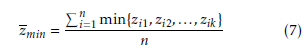where z_ik is the performance of a junction design alternative from the predicted set, given a combination of traffic demand pattern and size category i and n is the total number of these combinations to be evaluated. Using the rules, each combination i produces a predicted set of junction design alternatives. Each of these alternatives has a specific performance for the regarding objective. For each combination of i the minimum performance is used. These values are summed for all combinations of i and divided by the total number of combinations n. This is repeated for each objective and for both the Pareto optimal sets and the sets based on the existing and new rules.

A minor complication is the fact that sets can also contain the ’OTHER’ junction design alternative. As explained in section 2.2, for this combination of traffic demand pattern and size category, there was no junction design alternative with a delay below the chosen threshold value. Evidently, since the junction design is unknown, no performances can be determined for this alternative. Therefore, if a set contains an ’OTHER’ alternative, the regarding combination of traffic demand pattern and size category i is excluded from equation 7.

4. Cases

Junction design rules can be found in design manuals, which are usually issued by government agencies on a provincial, state or national level. For example, junction design rules are provided in design manuals for the following countries: Australia [21], Belgium [22], Germany [23, 24, 25], France [26], The Netherlands [27, 28, 29], UK [30] and USA [31, 32, 7, 2, 5, 33]. The availability and content of the rules is country specific. This is caused by the fact that policies, procedures, junction design alternatives, traffic modes, traffic behaviour and accepted modelling tools are very different by country. For example, in some countries turbo-roundabouts are generally accepted, whereas in other countries they are not (yet) considered as a viable alternative. Another example is that the same roundabout design can have a different operational and safety performance in different countries. It is not useful to determine universal junction design rules, but rather determine them for a specific region or country. We chose two case countries, being the United States of America (USA) and the Netherlands, mainly due to the availability of documented junction design rules and corresponding performance models. For both cases, first a short description of the existing rules is given, followed by a brief explanation of the existing rules that haven been chosen for comparison and the application of our approach for the specific case.

4.1. Case 1: United States of America

In this section we will explain the application of our approach as part of a junction design assessment process in the USA.

4.1.1. Existing rules

In the USA, junction design rules can be found in both national and state documents. Here, we will focus on the national level. Junction design rules are scattered over various junction design manuals and technical reports, published by TRB [2, 33], FHWA [34, 32] and AASHTO [31, 35]. A lot of rules require data generated by performance models and lie outside our research scope which aims to determine rules for the first stage of the junction design assessment process. The Manual on Uniform Traffic Control Devices (MUTD) [32] describes eight warrants that define conditions in which a traffic control signal is likely to improve junction safety, operations, or both. If a warrant is met, then signal control may be appropriate. Some warrants require volume based input data, such as eight, four or one hour volumes, while others require performance based data such as delay or the crash history or specific local data such as the area population. Various rules exist for the realisation of specific junction design alternatives and elements, such as volume thresholds for roundabouts or for the number of entry lanes required, e.g. [33]. An overall approach is also provided, combining the earlier mentioned warrants and various other rules in one method [2]. Not all warrants and rules are relevant and/or usable in order to determine a viable set of junction design alternatives. The rules had to be adapted to be used in this research, in order to make a fair comparison between existing and new rules. An extensive description of the existing rules that we used can be found in the Appendix.

4.1.2. Application of the approach

New junction design rules will be determined by using the approach as described in section 2. An important first step is to define the scope, where choices have to be made concerning the junction design alternatives, the traffic flow ranges, the objectives and the performance models to be considered. Table 3 shows the scope definition for this case.

The junction design attributes have been chosen to match the junction design types for the existing rules. Four main types are differentiated. The alternatives are based on the design alternatives mentioned in the underlying existing rules. When there are multiple approach lanes, different lane configurations are possible for the major and minor roads. Multiple variants are then differentiated, leading to 67 separate alternatives to be tested. Seven size categories are differentiated, which is necessary for the approach to avoid that only the largest junction design types are part of the Pareto optimal set and thus the rules to be determined. An overview of the junction design alternatives can be found in 10 in the Appendix.

Table 3: Scope definition for case 1: USA

Topic	Item	Choices
Junction design	Arms Main types Alternatives Variants	4 AWSC, TWSC, signalised, roundabout 21 67
	Size categories	7
	Attributes	Junction: Main type; Arm: Approach lane configuration, central reservation width, number of exit lanes, sign type, circulating lanes
Traffic flow	Units Modes Flows	Peak hour volumes (pcu/h) Motorised vehicles 12 turning flows for motorized vehicles
	Ranges	Total volume: 0-7000 (pcu/h),
Objectives	Objectives Measures	Operation, safety Volume weighted average delay (s), number of fatal-and-injury crashes per year
	Thresholds	Average delay ≤ 50 (s)
Models	Operation Safety	HCM 2010 methodologies HSM 2010 methodologies

Random traffic flow patterns are generated based on a total motorised volume ranging between 1 and 7000 (pcu/h). Two objectives and corresponding performance measures have been defined. Junction design alternatives with an average delay above 50 seconds are excluded from the choice sets.

The models used to determine the performances are static analytical based. The operational performance model is an implementation of the Highway Capacity Manual 2010 (HCM2010) methodologies [5]. For signalised junctions control settings (cycle time, green times) are determined (based on the traffic flow and junction design) which aim to minimise the average delay on the junction. The safety performance model is an implementation of the Highway Safety Manual 2010 (HSM2010) methodologies [35].

4.2. Case 2: The Netherlands

In this section we will explain the application of our approach as part of a junction design assessment process in the Netherlands.

4.2.1. Existing rules

In the Netherlands, junction design rules can be found in various publications of the CROW [36, 27, 28, 29]. Most rules are capacity thresholds, which means that they provide a value for the maximum allowed traffic volumes for a certain time interval, e.g. the total traffic volume on a junction or arm in a peak hour (pcu/h). Various tables are provided for various junction design types. Another, rather general but common rule, prescribes a preferred order in which main junction design types should be considered [28, 29]. The preferred order, being; roundabout, priority junction and signalised junction is based on the sustainable safety principle, in which roundabouts are considered (and proven to be) the safest junction design types. The rule dictates that a roundabout should be considered, unless it should be excluded for operational reasons. Furthermore, various design rules exist for specific design elements and/or junction design types. For example, a graphically represented rule which can be used to determine whether a single lane roundabout should be considered for a given combination of entry flow, conflicting circulating flow and crossing bicycle flow [36].

There is no overall (set of) junction design rule(s) available applicable for all relevant junction design alternatives and traffic modes. Therefore, we use a combination of rules from two source. The first source [27] provides two capacity thresholds for different types of junctions,ranging from single lane roundabouts, two lane roundabouts to turbo-roundabouts, priority junctions and signalised junctions. The first threshold represents the maximum allowed sum of all entry flows in a peak hour. The second threshold represents the sum of the entry flow and the (potentially) conflicting flow for one arm and is thus evaluated for each arm. If one of the threshold values is exceeded, then this junction design type is considered unsuitable to be taken into account for further research. The second source [29] provides the so-called Slop-criterion which calculates a value based on the (eight-hour) total volume on the major road, the (eight-hour) maximum volume of the minor roads and a set of parameters. If the resulting value exceeds a certain threshold value, a priority junction is no longer a viable solution. Using the (capacity) thresholds does not provide a set of viable junction design alternatives. However, the rule can be used to determine such a set. An extensive description of the existing rules that we used can be found in the Appendix.

Since bicycle flows are a substantial part of traffic flow in the Netherlands, it is desirable to reckon with these in the rules. However, since there are no existing rules for all junction design types, crossing bicycle flows will be reckoned with in the existing rules by simply adding them to the conflicting flow (1 bicycle = 0.2 pcu), which is used in various rules.

4.2.2.  Application of the approach

New junction design rules will be determined by using the approach as described in section 2. An important first step is to define the scope, where choices have to be made concerning the junction design alternatives, the traffic flow ranges and the objectives to be considered. Table 4 shows the scope definition for this case.

The junction design attributes have been chosen to match the junction design types for the existing rules. Four main types and 16 junction designs are differentiated. When there are multiple approach lanes, different lane configurations are possible for the major and minor roads. Multiple variants are then differentiated, leading to 42 separate alternatives to be tested. Five size categories are differentiated, which is necessary for the approach to avoid that only the largest junction design types are part of the Pareto optimal set and thus the rules to be determined. An overview of all junction design alternatives and variants can be found in the Appendix in Table 17.

Table 4: Scope definition for case 2: The Netherlands

Topic	Attribute	Choices
Junction design	Arms Main types Alternatives Alternatives	4 Equal, priority, signalised, roundabout 16 42
	Size categories	5
	Attributes	Junction: Main type; Arm: Approach lane configuration, central reservation width, number of exit lanes, sign type, number of opposed circulating lanes
Traffic flow	Units Modes Flows	Peak hour volumes (pcu/h) Motorised vehicles, bicycles 12 turning flows for motorised vehicles, 4 crossing flows bicycles
	Ranges	Total       motorised      volume:         1-7000 (pcu/h), total bicycle volume 0-500 (bicycles/h)
Objectives	Objectives Measures	Operation, safety, environment Volume weighted average delay (s), number of fatal-and-injury crashes per year, NOx/PM10 emission (g)
	Thresholds	Average delay ≤ 50 (s)
Models	Operation Safety Environment	Local static analytical models

Random traffic flow patterns are generated based on a total motorised volume ranging between 1 and 7000 (pcu/h) and a total bicycle volume ranging between 0 and 500 (bicycles/h). Three objectives and corresponding performance measures have been defined. Junction design alternatives with an average delay above 70 seconds are excluded from the choice sets.

The models used to determine the performances are static analytical based and were specially developed and tested for use in the Dutch practice [37]. The operational performance model is similar to the methodologies provided in the American HCM2010 [5] and the German HBS2015 [25], extended with new methods for (turbo)roundabouts and the effects of bicycle traffic. The safety performance model is similar to the American HSM2010 [35] methodologies, where parameters were adopted from [38] for local situations. The environmental performance model determines the emissions based on local emission substance factors multiplied by the queue on each lane [39, 3].

5. Results

In this section we will discuss the results. We will first consider the predictive accuracy of the existing and newly determined junction design rules. Next we will evaluate the performances of the predicted sets of viable junction designs. All results were determined with the test dataset.

5.1. Accuracy

Table 5 shows accuracy values for both the existing and new rules for both cases. The accuracy represents how good the rules can predict the Pareto optimal sets. The table shows values for sufficiency, similarity, equality and overestimation, according to equations 3-5. In addition to the accuracy values, the average set size is presented.

Table 5: Accuracy measures of existing and new rules for both cases

Item	Case 1			Case 2
	Existing	New	Existing		New
Sufficiency	0.311	0.905	0.845		0.899
Similarity	0.249	0.723	0.391		0.821
Equality	0.129	0.492	0.051		0.745
Overestimation	1.320	0.550	1.596		0.293
Average set size	1.857	1.741	2.606		1.242

The table shows that the new rules can better predict the Pareto optimal sets then the existing rules can. For both cases, the sufficiency values, being the measure for the predicted set at least containing the true (Pareto optimal) set, for the new rules are higher. For case 1 the difference is evident. The existing rules have a sufficiency rate of 31.1% where the new rules accomplish a 90.5%. For case 2, the difference in sufficiency rates is limited, with respectively 84.5% and 89.9% for the existing and new rules. However, there are big differences for the other measures. This is caused by the fact that the existing rules predict large sets, with an average set size of 2.606 and an average overestimation of 1.596. Larger sets have a higher change to at least contain the true set, which is reflected in the sufficiency value. However, equality, which reflects the rate at which the predicted set being equal to the true set, is extremely low. The rules are not discriminating enough, thus causing substantially more work in a later stage of the junction design assessment process. The new rules produce more equal and smaller sets.

The presented accuracy values in Table 5 are average values for the whole test set. In order to determine whether differences exist for different size or volume categories, differentiated results are presented in Table 6 and Table 7.

Table 6: Accuracy measures for the new rules differentiated by size category for both cases

Case	Size category	Sufficiency	Similarity	Equality	Overestimation
1	1	0.951	0.826	0.674	0.404
	2	0.899	0.860	0.807	0.182
	3	0.882	0.807	0.586	0.375
	4	0.882	0.747	0.594	0.604
	5	0.873	0.583	0.234	0.805
	6	0.933	0.578	0.216	0.840
	7	0.913	0.660	0.335	0.642
2	1	0.954	0.902	0.851	0.153
	2	0.949	0.844	0.723	0.285
	3	0.894	0.857	0.802	0.179
	4	0.870	0.760	0.678	0.437
	5	0.830	0.743	0.672	0.410

In Table 6, which shows the accuracy measures differentiated by size categories, it can be seen that sufficiency rates are fairly stable for all size categories. The values range between 87.3% and 95.1% for case

1 and between 83.0% and 95.4% for case 2. For case 2, equality rates are also relatively high. For case 1, these rates are lower for the higher size categories. This means that the new rules predict bigger sets, which also can be seen while looking at the overestimation values. This is not a big problem, since the overestimation is still limited and moreover, the similarity values, which represent an average set comparison, are still reasonably high.

In Table 7, which shows the accuracy measures differentiated by volume categories, a similar stable set of sufficiency rates can be seen for both cases.

Table 7: Accuracy measures for the new rules differentiated by volume category for both cases

Case     Volume category                       Sufficiency    Similarity        Equality          Overestimation (pcu/h)

Sufficiency rates are best for the lower and higher volume categories. The middle categories generally have the lowest sufficiency values. This can in part be explained by the fact that there are more junction design alternatives available for these volume categories. Moreover, as was the case for the size categories, the similarity values are again still reasonably high.

Generally, it can be concluded that the new rules have a much better accuracy then the existing rules and that there are no specific weaknesses concerning the accuracy values if they are differentiated for size and volume categories. The Pareto optimal sets can be predicted with a 90% accuracy.

5.2. Performance

Table 8 shows the average minimum performances for all objectives as has been defined in equation 7. The operational performance is expressed as volume weighted average delay (s), the safety performance as the number of fatal-and-injury crashes by year, and the environmental performance as the PM₁₀ emissions (g). The table shows the average minimum performances for respectively the Pareto optimal sets, the sets predicted by the existing rules and the sets predicted by the new rules. For a fair comparison, if any of the sets (Pareto, existing, new) only contains the ’OTHER’ junction design alternative, the regarding instance is excluded from the analysis, as was mentioned in section 3.2.

Table 8: Performances measures of existing and new rules for both cases

min	Pareto	Existing	New	Pareto	Existing	New
Operation	16.415	24.476	18.588	15.579	23.995	31.367
Safety	0.787	0.782	0.776	0.581	0.577	0.574
Environment				0.923	1.869	1.028

For case 1, the new rules show that the average minimum performance for both objectives is better (lower) in comparison with the existing rules. This means that the new rules produce sets of junction design alternatives which contain alternatives with a better (lower) performance for either operation, safety or a combination of one or more of these objectives. This was to be expected, since the sufficiency rate for the existing rules was only 31.1% for this case. On the other hand, the differences are not as big as those for the accuracy rates. The new rules provide an average reduction of 24% for operational and only 1% for safety performances in comparison with the existing rules. This is partly caused by the exclusion of instances for which one of the sets predicts a single ’OTHER’ junction design alternative. This was the case for 58% of the instances. A striking point is the fact that the average minimum safety performance for both the existing and the new rules is lower than that for the Pareto optimal set. This seems strange, since an alternative that has the minimum (optimal) performance for one objective is to be expected to be in the Pareto optimal set. This was true, however since we used a threshold value for the operational performance, some alternatives were excluded from the eventual set. When the new rules ’accidentally’ predicted these alternatives, the performance measures for these alternatives were yet reckoned with.

For case 2, the average minimum operational performance is better for the existing rules than for the new rules. This is primarily caused by the fact that the existing rules predict large sets, as was mentioned in the previous section, thereby increasing the change that the junction design alternative with the minimum performance is part of the predicted set. Moreover, the existing rules are specifically made to serve the operational objective. On the other hand, the average minimum performance for the new rules is rather high. Further analysis shows that there is a relatively small amount of wrongly predicted junction design alternatives which have very high values for the operational performance. Table 9 shows the number of instances for various delay classes.

Table 9: Number of instances by delay class for case 2

Delay class (s)	Pareto	Existing	New
< 25	5389	5224	5227
≥ 25 and < 50	1157	1183	1185
≥ 50 and < 70	459	498	480
≥ 70	0	70	113

When using median values instead of average, the operational performances for the Pareto, existing and new sets are respectively 7.145, 7.175 and 7.156. The performance values for the safety and environmental performances are better (lower) for the new rules. The new rules provide an average reduction of 1% for the safety performance and 45% for the environmental performance.

Generally, it can be concluded that the new rules predict junction design alternatives with either equal or better (lower) performances for all objectives.

6. Conclusions

In this study, we demonstrated the application of a new approach to determine junction design rules for use in the first stage of the junction design assessment process. The approach uses decision tree algorithms to determine decision trees based on modelled data. There is a need for quick design rules which need limited input data. Although some of these rules exist, their usability is limited due to inconsistencies in rules and non-transparency in combination with objectives. In this paper, we present an approach by which new and better junction design rules can be determined. The resulting rules can be used to predict a set of viable junction design alternatives for the first stage of the junction design assessment process. Moreover, the predicted set is in fact the Pareto optimal set of solutions for multiple objectives, e.g. regarding operational, safety and/or environmental impact. The Pareto optimal set of solutions always contains the best solution, whatever set of weights is used for different objectives in a later stage of the assessment process, thus handling multiple objectives in a straightforward manner.

The approach was applied and evaluated on cases in two different countries. Results show that for about 90% of the situations the Pareto optimal set can be predicted by the new rules, whereas existing rules hardly reach 35% or are not discriminating enough resulting in large set sizes, creating more work in later stages of the junction design assessment process. The new rules provide better performances for the non-operational objectives (safety and environment). Results for the operational performances were different for the two cases. Generally, the new rules produce better results with smaller predicted sets.

The major contribution of this paper is that it presents an approach to determine consistent and complete junction design rules based on modelled data in a transparent and systematic manner. Although some efforts have been made to determine junction design rules based on modelled data no generic and transferable method had been developed until now.

Conflict of Interest

The authors declare no conflict of interest.

Acknowledgment

Time New Roman, 10 Normal. Acknowledge your institute/ funder.

Appendix

In this appendix we provide a description of the junction design alternatives and existing junction design rules for respectively case 1 and 2. At the end of the appendix, an explanation of the variable notations is provided.

Case 1: United States

Table 10 shows the junction design alternatives used for this case.

Table 10: Junction design alternatives for case 1

A=AWSC-junction,T=TWSC-junction,S=signalised junction,

1R=one-lane roundabout,2R=two-lane roundabout

There are 21 junction design alternatives. Each alternative can be identified by the main type and the number of approach lanes on the major and minor road arms. Junction design alternative number 4, with id ’S21’ is a signalised junction with two approach lanes on the major road arms and one approach lane on the minor road arms. A description of the characters uses for the junction types is provided at the bottom of the table. The number of exit lanes is automatically determined, based on the number of approach lanes with a destination to the regarding arm. When there are multiple approach lanes, different lane configurations are possible. Multiple variants are then differentiated, e.g. three (3 times 1) variants for alternative number 4 and nine (3 times 3) variants for alternative number 15. In total 67 separate variants are defined. The junction design alternatives are grouped in seven size categories (Sc), based on the required space. The rules are based on the guidelines provided in [2]. We only use guidelines that refer to a specific junction design alternative. Rules referring to more detailed design elements, such as on-street parking, leftturn prohibition, lane length, right-turn radius and signal flash mode, are excluded. Obviously, we only use guidelines that need volume-based input. Guidelines that require performance-based input, such as delay or crash-history, are excluded, since we don’t want to run a model or perform an extensive survey in the first stage of the junction assessment process. The guidelines regarding signalised junctions in [2] are based on the so-called traffic signal warrants from [40]. These warrants have been updated over the years and therefore we use the most recent version from [32]. Most guidelines regarding stop-controlled junctions are presented as graphs. For these, different (linear, exponential, logarithmic, second-order polynomial) functions have been estimated to fit the lines in the graphs.

Table 11 shows which rules are applied for each size category (Sc). Each size category has a base set of viable junction design alternatives, corresponding to the definitions in Table 10. For each alternative in the base set it is evaluated whether it should be included (I) or excluded (E) from the base set. For each main type (A=AWSC-junction, T=TWSC-junction, S=signalised junction and R=roundabout), this is determined by one ore more rules. Each rule performs a check resulting in a true or false value. If true then that particular type is either included or excluded from the base set. Table 11 shows which rules cause inclusion or exclusion. As a starting point all alternatives are excluded. The rules are executed in the order as shown in Table 11. For example, for size category (Sc) 1, ’S11’ is excluded unless one of the rules S1-S4 provides a true value. Alternative ’T11’ is excluded unless rule T1 is true, but if one of the rules T2-T4 is true it is always excluded. Table 12 provides the conditions that are checked for each rule.

Table 11: Junction design rules for case 1: Application of rules by size category

Sc

Base set

Rules

S1

S2

S3

S4

A1

A2

T1

T2

T3

T4

T5

R1

1

{A11,T11,S11}

I

I

I

I

I

E

I

E

E

E

2

{T21,S21}

I

I

I

I

I

E

E

3

{T31,S31,T22,S22}

I

I

I

I

I

E

E

4

{T32,S32,S41,1R11}

I

I

I

I

I

I

5

{S33,S42}

I

I

I

I

6

{S43,S44,2R11}

I

I

I

I

I

7

{S64,2R21,2R22}

I

I

I

I

I

Table 12: Junction design rules for case 1: Rules and conditions

Code	Condition	Specifics
S1	qmas8 ≥ λS1a and qmix8 ≥ λS1b	Signal warrant 1a
S2	qmas8 ≥ λS2a and qmix8 ≥ λS2b	Signal warrant 1b
S3	qmas aqmix4 +λS3b	Signal warrant 2
S4	qmas aqmix1 +λS4b	Signal warrant 3
A1	qmas8 ≥ 300
A2	J = signal
T1	qmas
T2	qmi1 > λT 2ae( 0.001qmas1)	≥ 2 lanes on minor road
T3	qmao b	left-turn lane on major road
T4	qmar1 > 683.6e( 0.004qmas1)	right-turn lane on major road
T5	T3 and T4
R1	qtot24 ≥ 3600+9000lc(1+(81/50))−94pl

Tables 13, 14 and 15 provide parameter values for the λ that is used in various rules. Table 16 provides the volume conversion factors that were used to determine the volumes needed for the rules, based on the peak hour volume flows (pcu/h) that are used as base input. The variable notations are explained at the end of the appendix.

Table 13: Junction design rules for case 1: Parameters for rules S1-S4

lma	lmi	λS1a	λS1b	λS2a	λS2b	λS3a	λS3b	λS4a	λS4b
1	1	500	150	750	75	0.7697	573.8	0.7815	751.44
≥2	1	600	150	900	75	0.7689	659.11	0.7339	842.04
≥2	≥2	600	200	900	100	1.0226	881.44	0.9397	1076.4

Table 14: Junction design rules for case 1: Parameters for rule T2

pmir	λT 2a
≤ 0.35	550.67
> 0.35	641.80

Table 15: Junction design rules for case 1: Parameters for rule T3

pmal	λT 3a	λT 3b
< 0.075	-922.4	6157.0
0.075 − 0.124	-951.8	6046.6
0.125 − 0.174	-863.7	5369.8
0.175 − 0.299	-997.9	5849.3
≥ 0.300	-880.7	5362.9

Table 16: Volume conversion factors for the junction design rules of case 1

Volume	Units	Factor
Peak hour volume	pcu/h	1.00
Peak hour volume	veh/h	0.93
Four-hour volume	veh/h	0.78
Eight-hour volume	veh/h	0.67
Daily volume	veh/day	10.33

Case 2: The Netherlands

Table 17 shows the junction design alternatives used for this case. There are 16 junction design alternatives. As for case 1, each alternative can be identified by the main type and the number of approach lanes on the major and minor road arms. The characters referring to the main junction types are slightly different compared to case 1, and are provided at the bottom of the table. In total 42 separate variants are defined. The junction design alternatives are grouped in five size categories (Sc), based on the required space.

The rules are based on guidelines provided in [27] and [29]. There are three main types of rules. The first rule uses a threshold value for the total amount of traffic on the junction. Different threshold values are used for different junction types. The second rule checks a threshold value regarding the conflicting volume for each arm. If the threshold is exceeded for one of the arms, a specific type is not viable. The third rule is the so-called Slop-criterion, which is used to check whether a priority junction is still viable. Table

18 shows which rules are applied for each size category

(Sc).

Table 17: Junction design alternatives for case 2

E=equal junction,P=priority junction,S=signalised junction,

1R=one-lane roundabout,2R=two-lane roundabout,TR=turboroundabout

Table 18: Junction design rules for case 2: Application of rules by size category

Sc	Base set					Rules
		E1	E2	E3	P1	P2         P3	S1	S2	R1	R2
1	{E11,P11,S11}	E	E	E	E	E               E	E	E
2	{P21,P22,S21,S22}					E	E	E
3	{S33,1R11,2R11}						E	E	E	E
4	{S44,2R22,TR22}						E	E	E	E
5	{S66,TR23,TR33}						E	E	E	E

In this case, as a starting point all alternatives for a specific size category are included in the final set unless one of the applied rules for that specific alternatives returns a true value. Table 19 provides the conditions that are checked for each rule.

Table 19: Junction design rules for case 2: Rules and conditions

Code           Condition                                                                     Specifics

E1                q_tot1 > 1500                                                                   total volume threshold

E2               q_c > 1100                                                                              conflicting volume threshold

E3                      (q_mix8/β₁)×(−1+ ^p1+β₂q_mas8/q_mix8) > 1.33              Slop-criterion

P1                q_tot1 > 1500                                                                   total volume threshold

P2               q_c > 1100                                                                              conflicting volume threshold

P3                      (q_mix8/β₁)×(−1+ ^p1+β₂q_mas8/q_mix8) > 1.33              Slop-criterion

S1	qtot1 > λS1	total volume threshold
S2	qc > λS2	conflicting volume threshold
R1	qtot1 > λR1	total volume threshold
R2	qc > λR2	conflicting volume threshold

Table 20: Junction design rules for case 2: Parameters for rules E3,P3

lma	lmi	β1	β2
1	1	300	2.0
2	1	300	2.4
1	2	400	3.2
2	2	400	2.7

Tables 20,21 and 22 provide various parameter values for the rules. In this case only one volume conversion value is used in comparison with the peak hour volume (1.00). In order to obtain the eight-hour volume a factor of 0.63 is used.

Table 21: Junction design rules for case 2: Parameters for rules S1-S2

                                   lma          λS1               λS2

Table 22: Junction design rules for case 2: Parameters for rules R1-R2

Roundabout alternative	λR1	λR2
1R11	2000	1500
2R11	2200	1700
2R22	3500	2400
TR22	3500	2100
TR23	4000	2300
TR33	4500	2800

Notations

Variables:

qat	Vehicular traffic volume for turn(s) a and time unit t
λr	Parameter for rule r
pm	Percentage of traffic volume for movement m
lc	Number of circulating lanes on a roundabout
lma	Number of lanes for the major approach
lmi	Number of lanes for the minor approach
J	Junction type

Subscripts (a,t,m):

1           Peak hour volume 4 Four-hour volume

8 Eight-hour volume 24 Daily volume ma Major arm approach volume mao Major arm opposing volume (right-turn and through) mar Major arm right-turn volume mas Sum of approach volumes of both major arms mi Minor arm approach volume mir Minor arm turn-turn volume mix Maximum approach volume of both minor arms tot Sum of approach volumes of all arms l Left-turn movement volume c Conflicting volume for an arm

1.  E. M. Bezembinder, L. J. J. Wismans, and E. C. van Berkum. Constructing multi-labelled decision trees for junction design using the predicted probabilities. In Proceedings IEEE 20th International Conference on Intelligent Transportation Systems, Yokohama, Japan, October16-19 2017.
2.  TRB. Evaluating intersection improvements: An engineering study guide. NCHRP Report 457, Transportation Research Board of the National Academies, Washington D.C., United States, 2001.
3.  E. M. Bezembinder, L. J. J. Wismans, and E. C. van Berkum. Multi-objective assessment framework for intersection alternatives under different demands. In Proc. Transportation Research Board 95th Annual Meeting, Washington D.C., United States, January10-14 2016.
4.  L.D. Han, J-M Li, and T. Urbanik. Control-type selection at isolated intersections based on control delay under various demand levels. Transportation Research Record: Journal of the Transportation Research Board, 20701:109–116, 2008.
5.  TRB. Highway Capacity Manual 2010. Washington D.C., United States, 2010.
6.  B. J. Vitins and K. W. Axhausen. Shape grammars for intersection type choice in road network generation. In Proc. 12th Swiss Transportation Research Conference, Monte Verita/Ascona,Switzerland, May2-4 2012.
7.  TRB. Highway Capacity Manual 2000. Washington D.C., United States, 2000.
8.  A. Tarko, M. S. Azam, and M. Inerowicz. Operational performance of alternative types of intersections – a systematic comparison for indiana conditions. In Proc. 4th International Symposium on Highway Geometric Design, Valencia, Spain, June5-9 2010.
9.  E. M. Bezembinder, L. J. J. Wismans, and E. C. van Berkum. Using decision trees in order to determine intersection design rules. In Proc. Transportation Research Board 94th Annual Meeting, Washington D.C., United States, January11-15 2015.
10.  L. Rokach and O. Maimon. Data mining with decision trees. World Scientific Publising Co. Pre. Ltd., Singapore, 2008.
11.  S. Kotsiantis. Decision trees: a recent overview. Artificial Intelligence Review, 39:261–283, 2013.
12.  A. Clare and R. King. Knowledge discovery in multi-label phenotype data. In Proceedings of the 5th European Conference on PKDD, Freiburg, Germany, 2001.
13.  Y.L. Chen, C.L. Hsu, and S.C. Chou. Constructing a multivalued and multi-labelled decision tree. Expert Systems with Applications, 25:199–209, 2003.
14.  S.C. Chou and C.L. Hsu. Mmdt: a multi-valued and multilabeled decision tree classifier for data mining. Expert Systems with Applications, 28:799–812, 2005.
15.  H.Li, R. Zhao, J. Chen, and Y. Chang. Research on multi-valued and multi-labeled decision trees, pages 247–254. Springer Berlin Heidelberg, 2006.
16.  W. Yi, M. Lu, and Z. Liu. Multi-valued attribute and multilabeled data decision tree algorithm. International Journal of Machine Learning and Cybernetics, 2:67–74, 2011.
17.  W. Yi, L. Yan, M. Lu, and Z. Liu. A new multi-valued attribute and multi-labeled data decision tree algorithm. Information, 16(7A):4771–4780, 2013.
18.  E.F. Codd. Further normalization of the data base relational model, volume 6 of Courant computer science symposium, pages 33–64. NJ: Prentice-Hall, Englewood Cliffs, 1972.
19.  L. Breiman, J. Friedman, R. Olshen, and C.Stone. Classification and regression trees. Wadsworth International Group, Belmont, California, 1984.
20.  T. Brands. Multi-objective optimisation of multimodal passenger transportation networks. PhD thesis, University of Twente, Enschede, The Netherlands, 2015.
21.  Austroads. Guide to traffic management part 6: Intersections, interchanges and crossings. Technical report, Austroads, Sydney, Australia, 2013.
22.  AWV. Vadumecum veilige wegen en verkeer. Technical report, Vlaamse Overheid, Agentschap Wegen en Verkeer, Brussels, Belgium, 2009.
23.  FGSV. Richtlinien fr die anlage von stadstrassen: Rast06. Technical Report 200, Forschungsgesellschaft fr Strassen- und Verkehrswesen, Kln, Germany, 2007.
24.  FGSV. Richtlinien fr die anlage von landstrassen: Ral. Technical Report 201, Forschungsgesellschaft fr Strassen- und Verkehrswesen, Kln, Germany, 2013.
25.  FGSV. Handbuch fr die bemessung von strassenverkehrsanlagen. Technical Report 299, Forschungsgesellschaft fr Strassenund Verkehrswesen, Kln, Germany, 2015.
26.  SETRA. The design of interurban intersections on major roads. Technical report, Service d’tudes Techniques des Routes et Autoroutes, Bagneux Cedex, France, 2002.
27.  CROW. Turborotondes. Technical Report Publication 257, CROW, Ede, The Netherlands, 2008.
28.  CROW. Asvv 2012. Technical Report Publication 723, CROW, Ede, The Netherlands, 2012.
29.  CROW. Handboek wegontwerp 2013. Technical Report Publications 328-331, CROW, Ede, The Netherlands, 2013.
30.  HE. Design Manual for Roads and Bridges. London, England, online version march 2017 edition, 2017.
31.  AASHTO. A Policy on Geometric Design of Highways and Streets, 6th Edition. Washington D.C., United States, 2010.
32.  FHWA. Manual on uniform traffic control devices for streets and highways (mutcd). Technical Report 2009 Edition with Revisions 1 and 2, May 2012, Federal Highway Agency of the United States Department of Transportation, Washington D.C., United States, 2012.
33.  TRB. Roundabouts: An informational guide. NCHRP Report 672, Transportation Research Board of the National Academies, Washington D.C., United States, 2010.
34.  FHWA. Alternative intersections/interchanges: Informational report (aiir). Technical Report FHWA-HRT-09-060, FHWA, Washington D.C., United States, 2010.
35.  AASHTO. Highway Safety Manual. Washington D.C., United States, 2010.
36.  CROW. Eenheid in rotondes. Technical Report Publication 126, CROW, Ede, The Netherlands, 1998.
37.  E. M. Bezembinder. Junction modelling 2.0. Technical report, Windesheim, Zwolle, The Netherlands, 2018.
38.  A. Dijkstra. Enkele aspecten van verkeersveiligheid. Research report R-2014-21A, StichtingWetenschappelijk Onderzoek Verkeersveiligheid SWOV, Den Haag, The Netherlands, 2014.
39.  R. H. Gasthuis. Emission modelling on junctions in urban networks. Master’s thesis, University of Twente, Enschede, The Netherlands, 2015.
40. FHWA. Manual on uniform traffic control devices for streets and highways (mutcd). Technical report, Federal Highway Agency of the United States Department of Transportation, Washington D.C., United States, 2000.

(Click Here)

(Click Here)