1. Introduction

In recent years, Feedback linearization has been attracted a great deal of interesting research. It’s an approach designed to the nonlinear control systems, which based on the idea of transforming nonlinear dynamics into a linear form. The base idea of this technique is to algebraically transform a nonlinear dynamics system into a totally or partially linear one, so that linear control techniques can be applied. This notion can be used for both stabilization and tracking control objectives of SISO or MIMO systems, and has been successfully applied to a number of practical nonlinear control problems such as [1-4].

    In fact, this technique has been successfully implemented in several faisable applications of control, such as industrial robots, high performance aircraft, helicopters and biomedical dispositifs, more tasks used the methodology are being now well advanced in industry [5-6].

In this case, we applied this technique to lead the control for each joint of a robot manipulator that is has six degrees of freedom, which the equations of motion form a nonlinear, complex dynamic and multivariable system, then, we elaborated a PD linear controller for each decoupled linear subsystem to control the angular position of each joint of this robot arm for stabilization and tracking purposes. The obtained results in different simulations shown the efficiency of the derived approach [7].

   This paper is organized as follows: It is divided into five sections. In Section 2, a description of the input-output feedback linearization approach is detailed. In Section 3, a simplified dynamic model of a robot manipulator with six degrees of freedom is presented, the input-output feedback linearization method is applicated to the above robot and the construction of linear PD controller is derived. In Section 4, the simulation results are presented. Finally, the conclusion was elaborated in Section 5.

2. Input-Output feedback linearization for MIMO nonlinear system.

In this section, we discussed the approach of input-output feedback linearization of nonlinear systems, the central goal of feedback-linearization is to design a nonlinear-control-law as assumed that the inner-loop control is, in the most suitable case, precisely linearizes the nonlinear system after appropriate state space modification of coordinates [1]. The developer can then build an outer-loop-control in the new coordinates to obtain a linear relation between the output Y and the input V and to satisfy the traditional control design specifications such as tracking, disturbance rejection, as shown in Figure 1.

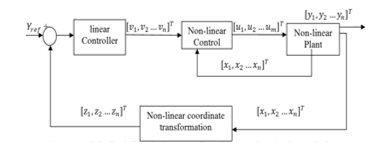Figure 1. Structure of Input-Output Feedback Linearization Approach.

     The basic condition for using feedback linearization method is nonlinear dynamic MIMO of n -order with p number of inputs and outputs described in the affine form;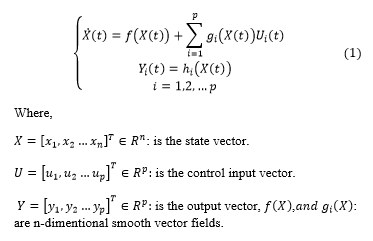

Where,

: is the state vector.

 is the control input vector.

   is the output vector, , : are n-dimentional smooth vector fields.

smooth nonlinear functions,with i=1,2…n.

Theorem1:

Let f: represent a smooth vector field on  and let

h : represent a scalar function. The Lie Derivative of h, with respect to f, denoted   is defined as [1-2].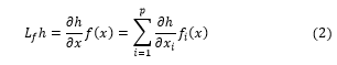

The Lie derivative is the directional derivative of h in the direction of f(x), in an equivalent way, the inner product of the gradient of h and f. We defined by the Lie Derivative of  with respect to f:

In general we define:

with

Theorem2:

The function  defined in a region  he is called difeomorphisme if it checks the following conditions:

Firstly, a diffeomorphism is a differentiable function whose inverse exists and is also differentiable. Second, we should assume that both the function and its inverse to be infinitely differentiable, such functions are usually referred to as  diffeomorphisms [3-4].

The diffeomorphism is used to transform one nonlinear system in another nonlinear system by making a change of variables of the form:

Where represents n variables;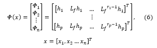

The goal is to obtain a linear relation between the inputs and the outputs by differentiating the outputs  until the inputs appear. Suppose that  is the smallest integer such that fully one of the inputs appears in  using this expression: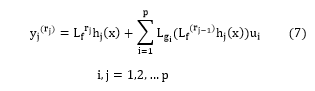

Where, and : Are the Lie derivatives of  respectively in the direction of f and g.

is the relative degree corresponding to the  output, it’s the number of necessary derivatives so that at least one of the inputs appear in the expression [5].

If expression  , for all i, then the inputs have not appeared in the derivation and it’s necessary to continu the derivation of the output .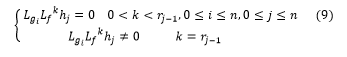

The system (1) has the relative degree (r) if it satisfies: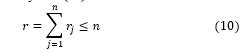

The total relative degree (r) was considered as the sum of all the relative degrees obtained using (7) and must be less than or equal to the order of the system (10):

To find the expression of the nonlinear control law U that allows to make the relationship linear between the input and the output [6], the expression (2) is rewritten in matrix form as:

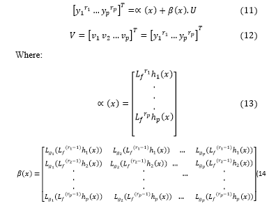If β (x) is not singular, then it is possible to define the input transformation “the nonlinear control law ” which has this form:

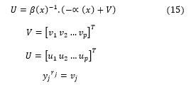
where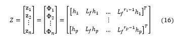

V: Is the new input vector. is called a decoupling control law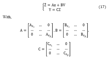

Is the invertible (pxp) matrix. Is called a decoupling matrix of the system.

2.1.  Non-linear coordinate transformation:

By applying the linearizing law to the system,we can transforme the nonlinear system into linear form [7-8]:

2.2.  Design of the new control vector V:

    The vector v is designed to according the control objectives, for the tracking problem considered, it must satisfy:

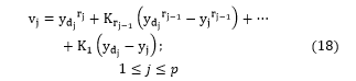 denote the imposed reference trajectories for the different outputs. If the are chosen so that the polynomial [9-10];

 are Hurwitz (has roots with negative real parts). Then it can be shown that the error , satisfied .

3. Input-Output feedback linearization approach applied to a robot manipulator with six degrees of freedom

3.1.  Dynamic modeling of a robot manipulator

   In this section, we have applied the proposed approach to a dynamic multivariable system which represent a robot arm with six degrees of freedom “EPSON C4”. This is an open chain kinematic manipulator robot consisting of seven rigid bodies interconnected by six revolute joints n = 6 as [11]. So, deriving the motion of robot is a complex task due to the nonlinearities present in this system and the large number of degrees of freedom [12-13]. Then, it is essential to understand exactly the dynamics of this interconnected chain of rigid bodies, to detemine the inverse dynamics model such as relation (19), we analyzed the evolution of motion of this mechanical non linear system by using the Euler-Lagrange equations, which is represented by the equation (20).

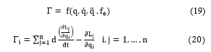where  depicting Torques, articular positions, velocities, accelerations and the external force.

  : Defines the lagrangian of the ^th link, which is the difference of the kinetic and potential energy, equal to  – .

and Define the kinetic and the potential energies of the ^th link.

The calculation of the kinetic energy;

In this section, we have calculated the total kinetic energy of the system which depends on the configuration and joint velocities, such that [13], then, it was described by the equation (21).

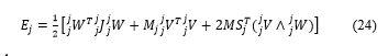
: means the kinetic energy of the link , which can be formulated such that (24). Firstly, we have calcuated the linear velocity and the angular velocity using the equations (22) and (23).

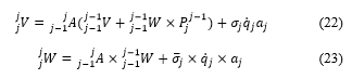  : The linear velocity, it is the derivative of the position vector .

: The angular velocity.

The initial conditions for a robot which the base is fixed, are

 = 0 and  = 0.

Then,we have expressed these relations (22) and (23) in Equation (24) as.

where

 :is the unit vector along axis .

,  et :are the inertial standard parameters.

 : is the mass of link

 :design the first moments of inertia of link  about the origin of the frame  It is equal to  = .

: is the inertial tensor matrix (3×3) of link  with respect to the frame , it is expressed by the matrix (25).

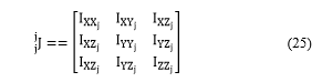and  represent the elements of the inertial tensor the symmetric matrix  of each link  which is expressed by the matrix (25), we have defined all these inertial parameters values in our recent work [14].

The calculation of the potential energy;

  In this section, we have represented the potential energy for a manipulator arm [14], which is written by the equation (26).

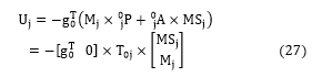
: Defines the potential energy of the link , which is expressed by the equation (27):

Then, we have followed the Euler-Lagrange formalism such that equation (20), we obtained the following relation (28):

where

A(q): Represents the matrix of kinetic energy (n × n), these elements are calculated as follows:

 is equal to the coefficient of  located in the expression of the kinetic energy.

–  is equal to the coefficient of

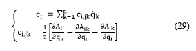
: Defines the vector of coriolis and centrifugal forces/torques (n × 1), these elements are calculated from the Christoffel symbol  such as system (29):

 Represents the vector of torques/forces of gravity, these elements are calculated as:

   The elements of A, C and Q are according to the geometric and inertial parameters of the mechanism. The dynamic equations of the robot form a system of n differential equations of the second order, coupled and nonlinear. Then, since the inertia matrix A is invertible for  we may solve for the acceleration  of the manipulator as [14].

With,
The angular position vector (6×1).

 The angular velocity vector (6×1).

 The angular acceleration vector (6×1).

  The input torques vector(6×1).

3.2. Application of the input-output feedback linearization approach to a robot manipulator with six degrees of freedom:

In this section, after we dermined the inverse dynamic model of the system [15-16], we used the equation of motion of the six-link of the rigid manipulator robot “EPSONC4” which represented by the relation (31) and we considered the state variables of the system defined in state space as;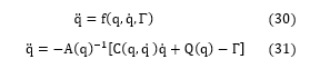

After derivation of the above state variables, we written the obtained system as;

Then, the affine form of nonlinear, multivariable and dynamic model of the robot manipulator is appeared which given by the following system (33):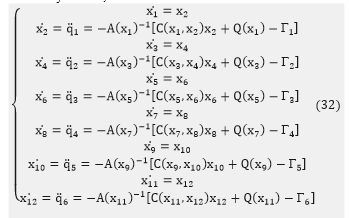

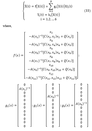
Links positions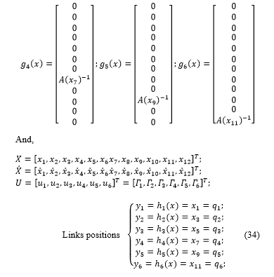

So, we made the derivation of each output  intel the inputs appeared in the expression and we computed the relative degrees  for each joint of the robot as follows [17-18];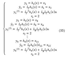

Therefore, the relative degree of each joint  is well defined and is equal to 2, so we computed the nonlinear control law of each joint of the system as this relation (36);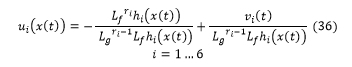

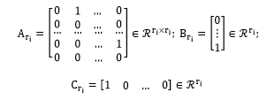
By using the nonlinear control law and diffeomorphic transformation given above, the nonlinear dynamic system with six degrees of freedom is converted into the following Brunovesky canonical form and simultaneously output decoupled [19].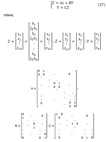

The above matrices A,B and C are of dimension respectively : .

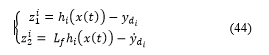
We note that, the obtained linear system (37) definied by six decoupled and linear subsystems that is has the following form (38), and i=1…6;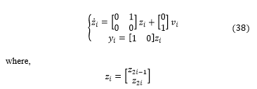

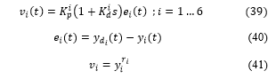
For the objective of linear control, we added to each subsystem a linear PD controller which has represented equation (39) as;

we obtained the relative degree for each subsystem as :

Then, we used the diffeomorphic transformation (16) presented above, we considered these relations for each SISO subsystem:

That is leads to the non-linear coordinate transformation given by:

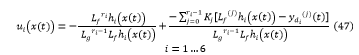
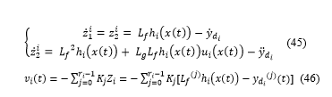So, we expressed the relation (46) in equation (36),we obtained:

Next, we expressed the equation (47) in the subsystem (45), the non linear subsystem (45) was transformed to a linear subsystem which expressed as relation (48):

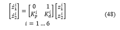The obtained linear subsystem consists of a second order system with linear output, that is can be computed the poles of the above subsystem as;

Where, : means damping ratio, :means natural frequency, for goal of stability we chosed the parameters of each PD controller applied to each subsystem as [19]:

4. Simulation Results

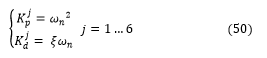
    In order to improve the efficiency of the proposed approach, we applied the above method of linearization to a robot manipulator which represent a non linear, decoupled and multivariable system. We imposed the sinusoidal signals as  and  which are represented inputs desired trajectories to each joint of the studied system. Therefore, the relative degrees  is well defined, we presented the simulation results depicting the output of each joint i=1…6 as shown in Figures 2,3,4,5,6,7,8-9.

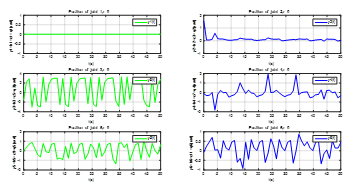Figure 2. The outputs plot of each joint, the relative degrees , i=1…6.

    Firstly, we made the simulation of the outputs of each joint of the robot,  the results are therefore given in Figure 2, we can see the non linearity of each subsystem. Second, we applied the Lie derivation to each output we shown the results presented in Figure 3 as.

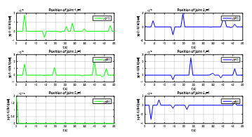Figure 3. The outputs plot of each joint, the relative degrees , i=1…6.

    In this case, the relative degrees equal to , , so no one input has been appeared, as shown in Figure 3, the system still non linear. Finally, we made the derivation again of each recent output  the inputs appeared in the expression and we computed the final relative degrees  for each joint of the robot, , the results was illustrated in these Figures 4,5,6,7,8-9.

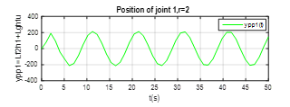Figure 4. The output plot of the joint 1, the relative degree .

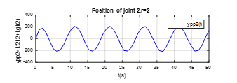Figure 5. The output plot of the joint 2, the relative degree .

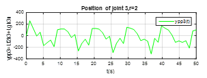Figure 6. The output plot of the joint 3, the relative degree .

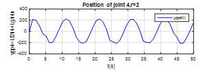Figure 7. The output plot of the joint 4, the relative degree .

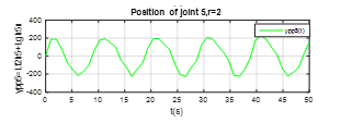Figure 8. The output plot of the joint 5, the relative degree .

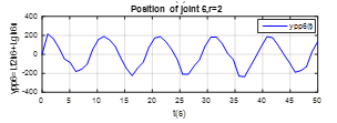Figure 9. The output plot of the joint 6, the relative degree .

These Figures 4,5,6,7,8-9 shown that the output of each SISO subsystem asymptotically tracks the sinusoidal input trajectory with minimum of oscillation and the efficiency of the studied approach.

5.  Conclusion

   In this paper, the input-output feedback linearization approach is presented which is a way of algebraically transforming nonlinear, multivaribles, complex and dynamics systems into linear ones, so we can be applied linear control, this technique has attracted lots of research in recent years. For that we applied this proposed approach to derive the control of a robot manipulator with six degrees of freedom which followed two major steps. Firstly, by using the above approach and diffeomorphic transformation, we converted the non linear and decoupled dynamics model of the robot to linear system. Then, we designed a linear PD control law for each decoupled subsystem to control the angular position of each joint of this robot for tracking purposes. Finally, the obtained results in different simulations illustrated the accuracy of the proposed approach.

1. MW. Spong, S.Hutchinson, and M. Vidyasagar. Robot Dynamics and Control , Second Edition. January 28, 2004.
2.  J.-J. Slotine & W. Li, Applied Nonlinear Control, Prentice-Hall, Englewood Cliffs, NJ, 1991.
3.  A. Isidori. Nonlinear Control Systems. Springer Verlag, 1989.
4.  H. Khalil. Nonlinear Systems. Prentice Hall, Upper Saddle River, Second Edition, 1996.
5.  J.Hauser,S.Sastry, and P.Kokolovic,“Non linear control via approximate Input_Output Linearization,The Ball and Beam Exemple”. IEEE Transactions onAutomatic Control ,Vol 37,No.3 March 1992.
6.  E.D. Sontag,M. Thoma,A. Isidori and J.H. van Schuppen. Nonlinear and Adaptive Control with Applications, 2008 Springer-Verlag London Limited.
7.  H. Nijmeijer and A. J. van der Schaft, Nonlinear Dynamical Control
   Systems, Springer-Verlag, New York, 1990.
8.  M. Vidyasagar. Nonlinear Systems Analysis. Prentice Hall,Second Edition, 1993.
9.  K.M. Hangos, J. Bokor et G. Szederkényi, Analysis and Control of Nonlinear Process Systems, Springer-Verlag London Limited, 2004.
10.  J.HAUSER, SH. SASTRY and G. MEYER. “Nonlinear Control Design for Slightly Non minimum Phase Systems: Application to V/STOL Aircraft”. International Federation of Automatic Control. Vol. 28, No. 4, pp. 665-679, 1992.
11.  W.Ghozlane and J.Knani.“Modelling and Simulation Using Mathematical and CAD Model of a Robot with Six Degrees of Freedom,”CEIT-2016, 4thInternational Conference on Control Engineering & Information Technology on IEEE.16-18 December 2016-Hammamet, Tunisia.
12.  B.Siciliano and O. Khatib, Handbook of Robotics: Springer, 2007.
13.  W. Khalil and E. Dombre, Modeling Identification and Control of Robots, Hermes Penton London, 2002.
14.  Thomas R. Kurfess, Robotics and Automation Handbook, CRC press, 2005.
15.  Y . L . Chen: “ Nonlinear Feedback and Computer Control of Robot Arms”. D.Sc. Dissertation, Washington University, St. Louis 1984.
16.  V.D. Yurkevich, Design of Nonlinear Control Systems with the Highest Derivative in Feedback,World Scientific Publishing, 2004.
17.  Frank L.Lewis, Robot dynamics and control, in robot Handbook: CRC press, 1999.
18.  L. Sciavicco and B. Siciliano, Modeling and control of robot manipulators, 2nd edition, Springer-Verlag London Limited, 2000.
19.  C.T.Leondes. Control and Dynamic Systems,Advances In Theory and Applications, part 1 of 2,USA,1991.
20.  Zakaria, M. Z., Jamaluddin, H., Ahmad, R. & Loghmanian, S. M. R. (2010). “Multiobjective Evolutionary Algorithm Approach in Modeling Discrete-Time Multivariable Dynamics Systems”. Computational Intelligence, Modelling and Simulation (CIMSiM), 2010 Second International Conference on, Bali, Indonesia. 28-30 Sept. 2010. 65-70.
21.  Zakaria, M. Z., Jamaluddin, H., Ahmad, R. & Loghmanian, S. M. R. (2012). “Comparison between Multi-Objective and Single-Objective Optimization for the Modeling of Dynamic Systems”. Journal of Systems and Control Engineering, Part I. Proc. Instn. Mech. Engrs., 226 (7): 994-1005.

(Click Here)

(Click Here)