1. Introduction

This paper is an extension of a previous work originally presented at the 2017 International Conference on Network and Service Management (CNSM2017) [1]. User-generated content is growing exponentially. From 30 Zettabytes (ZB) of content generated in 2017, it is foreseen to reach 160 ZB by 2025 [2]. Although end-users create most of this content, with the widespread use of the Internet of Things (IoT) and the advances in cloud technologies, content generation will also increase at the core of the network. It is also worth noting that in 2017 approximately 40% of the content was stored in enterprise storages [2], but due to the paradigm shift from expensive and large data-centers to cloud-based virtualized infrastructures, it is also projected to increase to 60% by 2025. The massive scaling and flexibility required in those infrastructures will demand more efficient ways to handle the additional traffic.

At the outlook of such demanding requirements, Distributed Storage Systems (DSS) became more popular, since they provide highly reliable services by networking nodes to provide enhanced storage [3]. Over the years, DSS has progressively achieved better performance by improving propagation and recovery methods, from simple replication to more advanced techniques [4,5]. However, little attention has been paid to improvements at the network level, as they still rely on legacy techniques.

To cope with the increasing need for efficient storage managed by DSS, in this paper, we propose a network control method that is capable of handling the generated traffic by specific DSS tasks. The proposed method is based on Software Defined Networking (SDN) [6], which separates the control plane from the data plane and will allow a more flexible programmable network.　The contribution of this paper is to show the potential of applying this paradigm to improve DSS performance. Furthermore, we describe the inherent problems of DSS when using legacy techniques in Section 2, and the minimum requirements that DSSs demand from the network perspective, namely aggregated bandwidth and practical use of resource. Based on those requirements, we designed the proposed method as described in Section 3, whose main strength is its simplicity. More concretely, we define a solution to handle the bandwidth aggregation called on-demand inverse multiplexing, and we detail the solution for the practical use of resources called multipath hybrid load balancing.

To test the feasibility of the proposed method, in Section 4 we evaluated the implementation of typical DSS scenarios, the results showed that our method outperforms traditional ones, and is capable of delivering the required features by DSS.

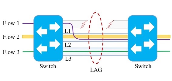Figure 1: Programmability problem with LAG

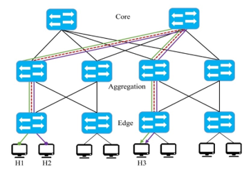Figure 2: Traffic congestion issue in DCNs

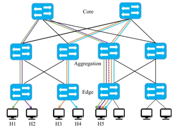Figure 3: The last-mile bottleneck issue in DCNs

2. Related Work

2.1.  Problem Description with Legacy Networking Techniques

To the best of our knowledge, solutions that combine features of both technologies (DSS and SDN) have not been fully explored yet, however, in this section we present related work on individual features.

Initially, we should mention that there are two minimum requirements DSS will need from the networking perspective, namely: aggregated bandwidth and practical use of resources. In this sub-section, we describe the specific problems with legacy techniques when applied to DSS regarding these two aspects.

In the case of bandwidth aggregation, since DDS nodes might be allocated in different storage servers, a bottleneck is created at the server gateway when various clients try to access it at the same time, due to the limited bandwidth of a single link. Kaneko et al. [7] tried to overcome this problem by using Link Aggregation (LAG) [8], which allows bandwidth aggregation by grouping a limited number of physical links as a single logical bundle. LAG offers communication resilience by redirecting the incoming traffic to another active link in case of failure. However, there is no control on the selection process, e.g., in the simple LAG deployment depicted in Figure 1, three links (L1, L2, and L3) are grouped in a single bundle, if L1 fails then the protocol redirects the traffic to another link, but the traffic may well be sent through the most congested link (L2) instead of the L3 which has less traffic. Moreover, for a link to be part of a bundle, all of them need to have the same configuration, and it is limited to a hard-coded number of links, which significantly limits the flexibility of the system.

In the second case, namely the practical use of resources, DSSs are typically deployed on Data Center Networks (DCNs) using common topologies, such as a three-layer non-blocking fully populated network (FPN) or three-layer fat-tree network (FTN) [9]. In these environments, network traffic management is usually leveraged to techniques such as Equal Cost Multipath (ECMP) [10]. However, ECMP is not efficient regarding resource usage, and since DSS clients access several storages concurrently, congestion mostly occurs at some segments of the network. Additionally, since it is limited to legacy protocols such as Spanning Tree Protocol (STP), it will prune redundant links, which can be used for creating alternative paths. For example, in the topology shown in Figure 2, if two flows go from H1 and H2 to H3, some routes might be preferred (e.g., the red dashed path), despite the availability of other paths. Moreover, as shown in Figure 3, a bottleneck is generated at the segment nearest to the end-device, for instance, if H5 have to reply flows from requests send by H1-H4, the link connected to the nearest switch will be highly congested (i.e., red dashed path). Apart from the number of flows going through a single link, that particular segment of the topology the connection speeds are not as fast as they are in the core, we call this problem “last-mile bottleneck.”

To sum up, legacy techniques cannot provide DSS with neither aggregated bandwidth or efficient use of resources due to the last-mile bottleneck issue, and limitations with end-to-end routing programmability with techniques such as ECMP.

2.2. Related work on SDN-based Multipath Load-balancing

The primary task towards a resource-efficient method is to balance the load among the available resources, and using multiple paths is a practical way to relieve the network traffic. Thus, in this section, we present load balancing solutions that focus on multipath solutions using SDN.

Initially, it is worth noting that load balancing is a topic that has been extensively explored for decades, but SDN-based solutions are relatively more recent. SDN-based load balancing can be categorized depending on their architecture in Centralized and Distributed [11], we focus on the centralized architectures wherein the management is performed in the data plane by a central controller that has an overview of the entire network. In this context, a pioneer work was Hedera, a dynamic flow scheduling for DCN capable of balancing the load among the available routes. The main contribution of the authors is the introduction of two placement heuristics to allocates flows, and the estimation of flow demands that uses OpenFlow (OF) for routing control. However, the authors did not consider last-mile bottlenecks nor the load on the server side.

OLiMPS [13] is a real implementation of Multipath TCP (MPTCP) [14] in an intercontinental OF-network that achieved high throughput. The drawback of this work is that, as other solutions [15, 16], they rely on MPTCP, which is an experimental protocol capable of handling resource pooling using multiple paths. However, the inherent problem is that it needs modifications in the end-point kernel. To avoid this restriction, Banfi et al. [17] presented MPSDN, a multipath packet forwarding solution for aggregated bandwidth, and load balancing that achieves similar results to MPTCP with the added value of not requiring end-point modifications. Their main contribution is the idea of including a threshold called Maximum Delay Imbalance (MDI), used to place flows in paths. However, even if they do not require end-point modification, they need to modify Open Virtual Switch (OVS).

DiffFlow [18] used a selection mechanism to handle flows in a DCN, so that short flows will be handled by ECMP and long ones using a process called Random Packet Spraying (RPS). However, by partially relying on ECMP they inherit the same issues concerning the use of resources.

Li and Pan [19] proposed a dynamic routing algorithm with load balancing for Fat-tree topology in OpenFlow based DCN. Their flow distribution strategy provided multiple alternative paths from a pair of end nodes and placed the flow to the one with the highest bandwidth. However, the hop-by-hop recursive calculation overlooked the available bandwidth of the entire network. A similar approach was presented by Izumi et al. [20], who proposed a dynamic multipath routing to enhance network performance, they introduce an index based on the risk and the use parallel data transmission and distribute the traffic using multiple paths. Dinh et al. [21] also presented a dynamic multipath routing, capable of selecting k-paths to distribute the traffic based on the load of the links; however, they only handled the initial assignment, and the selection of the number of paths is unclear.

Finally, Tang et al. [9] present an OF-based scheduling scheme that dynamically balances the network load in data centers. Their approach aimed to maximize the throughput by designing a heuristic based on the available resources in the network. A significant contribution of their work is that they present a theoretical model for load-balancing and specific metrics for network utilization and load imbalance. The drawback, however, is that they heavily rely on the use of a pre-calculated table (ToR Switch-to-ToR Switch Path Table S2SPT) for path selection, which dramatically limits the dynamicity in case of real implementation, as the computation time will increase if the number of links is relatively high. Moreover, they are still subject of the last-mile bottleneck problem due to the limitation in the DCN topology.

2.3. Target Issues

From the related work presented in the preceding sub-sections, and considering DSS requirements, we summarize our target issues as follows.

(P1) Last-mile bottleneck: Links have lower connection speeds at layers closer to the end-device in a DCN topology causes a network bottleneck. Therefore, DSS performance will be limited when performing parallel tasks.

(P2) Limited use of multipath routing: Despite the available redundant links in the topology, paths from end-to-end nodes are usually mapped as single-paths via some preferred routes, this provokes unnecessary congestion in specific segments of the network.

 (P3) Load Imbalance: Due to the limited use of the available resources DSS neither the network nor the servers are used in a balanced manner. The existing solutions focus on either one of those aspects, which leads to overlooking the importance of both variables for an effective control method.

3. SDN-based Network Control Method for Distributed Storage Systems

3.1    Motivating example

We describe the proposed SDN-based network control method to solve the problems described above. However, before describing the proposed approach, let us consider a simple scenario of a DSS process.

Suppose we have a DSS that uses network codes [3] to recover failed nodes. In this scenario, the information of a node (D) is fragmented into p=4 pieces (p₁, p₂, p₃, p₄) stored in different nodes from the set of nodes (N), such that any piece can be reconstructed from any k=3 pieces in N, but it needs the four pieces to recover D. If a node fails, the DSS needs to conduct two processes, namely, regenerate the piece and resume the primary data transmission.

The recovery process is described in Figure 4. Initially, D collects information from p₁, p₂, p₃, and p₄, but imagine p₄ fails; then the system needs to identify and locate the other pieces (p₁, p₂, and p₃)_, establish the corresponding recovery links (marked with dashed lines) and transfer the recovery data from the surviving pieces to a new node (p₄’). Once the transmission of the regenerated piece is over, the newly created piece (p₄’) will need to continue the primary data transmission, to do so, the system needs to identify the location of the new piece, establish the new link (blue line), and resume.

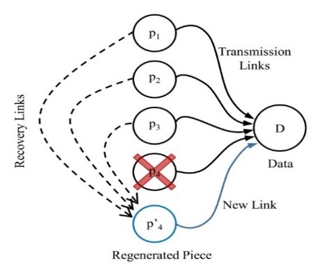Figure 4: Sample process in DSS

As observed, even in this small example, various processes occur from the networking point of view. Needless to say that the efficiency of the DSS will depend on how fast a node can be recovered and how efficiently uses the resources.

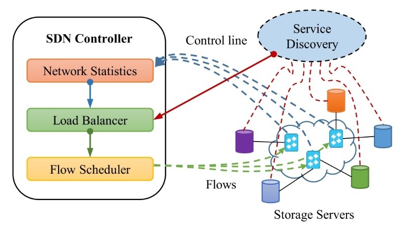Figure 5: Overview of the Proposed Method

3.2    Overview of the Proposal

To solve the target issues, we describe the proposed SDN-based Network Control Method for DSS. The overall scheme is depicted in Figure 5. As observed, the architecture consists of a centralized SDN controller that is comprised by three internal modules: Network Statistics, Load Balancer, and Flow Scheduler; additionally, an external module (Service Discovery) interacts with the controller and the storage servers connected in the underlying network. The role of each of these modules is described as follows:

• Service Discovery – this module is in charge of tracking the status of all the storage servers. This information includes the physical load of each of the servers (g., memory, CPU, number of processes being served), and the specific DSS configuration (i.e., the number of pieces and their location). The interaction with the SDN Controller is direct, and the status is sent when requested.

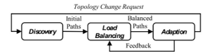Figure 6: Load Balancing Steps

• Network Statistics – periodically collects network statistics of the entire network, e., network topology changes, transmitted and received packets per port. This polling process will allow having an overview of the whole network infrastructure before calculating the appropriate paths. Although the polling happens periodically, it can also be triggered directly by request. We use this information to calculate parameters such as the available bandwidth (1)

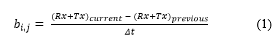• Figure 9: Sample hybrid load balancing (Final state)Load Balancer – this is the central module in charge of calculating the paths based on the information collected by the Service Discovery and Network Statistics The primary goal of this module is to distribute the traffic among the available paths based on not only the state of the network but also the load of the storages containing the required pieces. The overall process is subdivided into three phases, namely Discovery, Load Balancing, and Adaption (as depicted in Figure 6). In brief, once the request is sent from a source, in the Discovery phase, this module calculates the available paths from source to destination with a process we call on-demand inverse multiplexing (described in Section 3.3). Then, based on the current status of both network and storage servers, in the Load-balancing phase, a process we call hybrid Multipath Load-balancing assigns the paths that best suit the request. Finally, in the Adaption phase, once the transmission has started the status is updated periodically in case better routes become available or if any change occurred in the topology. The main load-balancing procedure is described in Algorithm 1, where a control loop checks if there has been any change in the topology within a fixed period. As observed, the function adjustWeights() in line 8, requests an update from the Network Statistics module, and in line 9 the function balanceTraffic() is in charge of performing the load-balancing.
• Flow Scheduler – once the most suitable paths have been selected, this module writes the flow rules into the specific network devices that take part in the transmission process.

Algorithm 1: Topology Monitor

1:    function monitorTopology (); 2:    startTimer(t); 5:    do 6:         if hasTimeElapsed() then 7:               if hasTopologyChanged() then 8:                      adjustWeights(), 9:                      balanceTraffic(client, Servers, NW), 10:             else restartTimer() then 11:             end 12:       else addTimeSpan(); 13:       end 14: While true;

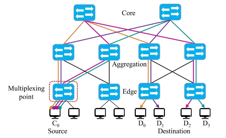Figure 7: On-demand Inverse Multiplexing

3.3    On-demand Inverse Multiplexing

As mentioned in the previous subsection, the initial step towards an effective network control is the path discovery and traffic distribution. In this section, we describe a process we called On-demand Inverse Multiplexing. Initially, it is worth noting that inverse multiplexing was explored in the past [22] and mainly used for bandwidth aggregation. It refers to the simple process of sending traffic over multiple paths. In essence, our particular contribution is the idea of distributing the traffic among a specific number of paths (k), which depend on the requirements in a particular DSS configuration. However, in a typical DCN deployment only single links are assigned from device-to-device; moreover, connections at the last layer in the topology are usually low-speed connections, which create a phenomenon we call a last-mile bottleneck.  To solve this problem, we propose to augment the topology by using parallel connections from the layer closest to the end-devices (edge layer) to the next hop (aggregation layer). This topology augmentation is central for our overall proposal and would involve the overprovision of links according to the particular configuration of the DSS, i.e., setup n links if the system split data in a maximum of n pieces. Although it is not a common suggestion, organizations still prefer to use various cheap links instead of expensive limited services, such as MPLS or single fat-line [23] due to the cost constraints. Note that, by performing this augmentation, the power consumption of the involved network devices will increase proportionally to the number of parallel connections, therefore, it is necessary to think of a strategy that is capable of reaching a tradeoff between the performance and the power consumptions, however, such a strategy is out of the scope of this paper.

To illustrate the implementation of the on-demand inverse multiplexing process, let us consider the scenario depicted in Figure 7, in this simple deployment, a Fat-tree fully-connected topology comprises three layers (Edge, Aggregation, and Core). Furthermore, assume the particular DSS uses four pieces out of 5 to regenerate as the maximum level of division. In this case, the number of links that the network needs to provision from the edge to the aggregation layer is four. Of course, the augmentation need not be among each device, but only in those particular segments wherein the requirements are higher and can be configured statically or calculated on-demand based on the configuration in the DSS gathered by the Service Discovery module.

Once we have the infrastructure prepared, the remaining process works as follows. Consider again the scenario depicted in Figure 7, where we emulate the data recovery which will be allocated in a storage server (C₀), the pieces needed for recovery are located in different servers (D₀, D₁, D₂, D₃). Therefore, in this simple example, the number of parallel links needed are k=4 paths. When the request arrives at the multiplexing point (the closest Top of Rack TOR switch), the controller calculates the appropriate number of paths (k) based on the information at the Service Discovery module and the current state of the network captured by the Network Statistics module.

To solve the initial path discovery, we calculate the Maximum Disjoint Paths (MDP) by a process described in Algorithm 2. This process, which is the initial step of this work and was introduced in [1], calculates the MDPs by an adapted version of the Suurballe’s [24] algorithm which calculates the path candidates. Note that we use a multigraph G = (V, E), where V is the set of network devices (switches), and E is the set of links. Since it is a multigraph, more than a single link can connect two nodes in the set V.  We assume that the bandwidth (b_i) for each edge is symmetric, which means that both the uplink and the downlink are the same. Moreover, each edge has a cost µ_{u, v} as shown in (2), where B is the set of all individual bandwidths b_i. This value is updated periodically by the Network Statistics module.

Algorithm 2: Path selection algorithm to find the kmax disjoint paths from source to destination

1:    function selectKPaths (s, t, k, G); Input  : s, t, k, G(the Vthe ,E) Output: Set of k path candidates P 2:    P ← Ø; 3:    currentPath ← Ø; 4:    nPath ← 1; 5:    do 6:         if nPath > 1 then 7:               adjustWeights (P[nPath-2]), 8:         end 9:         currentPath ← getDijkstraShortestPath(s,t) 10:       if currentPath ≠ Ø then 11:             nPath++; 12:             P.add(currentPath); 13:       end 14: While currentPath ≠ Ø and nPath ≤ k 15: return P

3.4    Hybrid Multipath Load-balancing

This part of the paper was partially presented in a previous work [25]. Usually, load-balancing techniques focus on either server or network load. In the proposed method, we consider both variables to balance the traffic, and that is why we call it hybrid. Moreover, since the topology was augmented with parallel links, it is necessary to take into account multiple paths to balance the traffic. The main procedure is described in Algorithm 3. Initially, from a pool of servers S, the lookupServers function (line 2) searches for the server candidates which can provide the required service (e.g., in the case of a regeneration process in DSS, it locates the nodes containing the pieces necessary to regenerate the current piece), which are then ordered based on the load of the node. In line 8, we search k alternative paths from the source c to each of the server candidates s that can provide the service. In line 9, the function assignPaths calculates the minimum combination of server and path cost. It is worth noting that, based on initial experimentation, the difference in overall cost from all the paths should be less than 25% otherwise the transmission will be delayed in the paths that have costs with the higher difference. This process will guaranty that the distribution is homogeneous in both, the network and servers. Finally, once the destination servers have been identified and the paths selected, the function writeFlows in line 11 will send the balanced paths to the Flow Scheduler module, which sends the instructions to the network devices involved in the path.

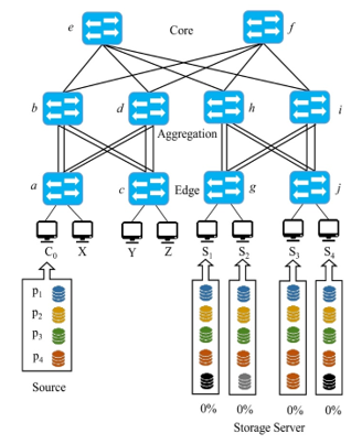Figure 8: Sample hybrid load balancing (Initial state)

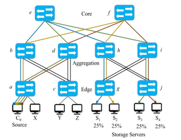Figure 9: Sample hybrid load balancing (Final state)

Algorithm 3: Hybrid Load Balancing Algorithm to calculate the best paths

1:    function balanceTraffic (c, S, G); Input  : Source, set of Servers, G(V,E) 2:    serverCandidates ← lookupServers(c,S); 5:    if isNotEmpty(serverCandidates) then 6:         foreach s in serverCandidates do 7:            k← s.lenght 8:            Candidates ← selectKPaths(c,s,k,G) 9:            BalancedPaths←assignPaths(c,Candidates), 10:       end 11:       writeFlows (BalancedPaths); 14: end

To illustrate the selection process, consider the contrived topology depicted in Figure 8. In this particular example, the features of the system are as follows:

• C₀ is a newly created node that needs to restore the data, to do so, it requires four pieces (p₁, p₂, p₃, and p₄)
• From the edge layer, there are two connections to the aggregation layer
• All links in the topology have weight=1
• None of the servers have any activity yet, and therefore the load is 0%.
• The storage servers that contain the replicas, among others, C₀ are S₁, S₂, S₃, S₄
• Each request consumes 25% of the server resources, and 100% of the link capacity, and therefore only one of the request can be served per path

When the recovery process starts, the lookupServers function will identify that S₁-S₄ have the pieces and their location, and all the candidates will be generated in pairs {(C₀, S₁), (C₀, S₂), (C₀, S₃), (C₀, S₄)} and since there are four pieces (p₁, p₂, p₃, and p₄) the function selectKPaths will search for four paths between each pair. Then the selection process in function assignPaths will start assigning the appropriate paths. For example, p₁ in C₀ to S₁, via the path: a →b→ e→ h→ g, adjust the weights and the load percentages and continue the process recursively until all the pieces have a service provider; the final result will look as shown in Figure 9, in which all the servers have a perfect balance, and the network traffic is evenly distributed among the available paths. Of course, this is not the unique process, neither are the request homogeneous, therefore, in case another process starts, i.e., from sources X, Y, or Z the values will vary in the service providers and the network load.

Note that this is just the initial assignment, but in case there is a change in the topology (e.g., a link disconnection, or a network device fails), the whole process needs to adapt and restart the process. In the proposed method, the adaption can happen proactively and reactively. In the first case, as shown in Algorithm 1 in Section 3.2, a timer determines how frequent the system needs to control the changes. Although fail-tolerance is not the focus of this paper, the value needs to have a trade-off between performance and service resilience, since having a small refresh time in the order of milliseconds would offer better service resilience at the cost of performance due to the constant polling. In case of reactive adaption, which is an event-based procedure triggered by any change in the topology during the transmission, the system needs to recalculate all the paths in the affected segments.

3.5    Implementation

Based on the overall scheme presented in the previous sub-sections, we implemented the proposed approach using a commonly used SDN controller OpenDaylight[1] Belirium-SR3 (ODL), OF 1.3 as the communication protocol, and OVS as the back-end deployment.

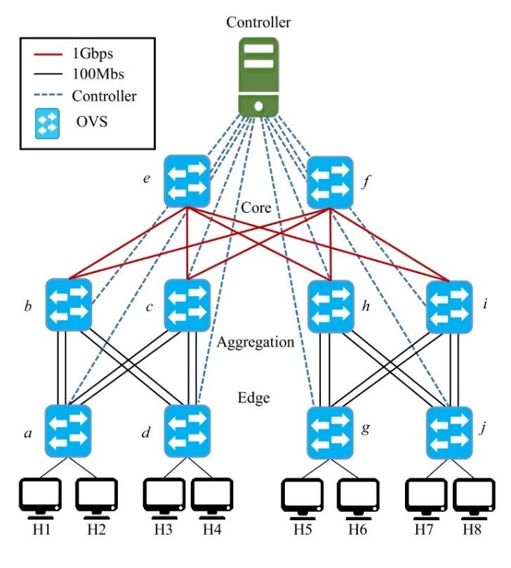Figure 10: Testbed Experiments

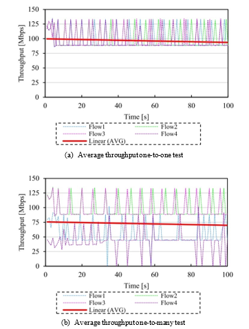Figure 11: Results average throughput

Each of the modules was implemented as part of the controller as follows. The Service Discovery module provides a global record of servers’ status so that every time a new request arrives at the controller it verifies and updates the status of all the servers involved, and when the transmission is over the status is once again updated. This module could keep track of various parameters, but for simplicity in the current implementation, we only use the following attributes.

ServerID, MaxLoad, Ports[ID, CurrentRequest, Location]

MaxLoad is the maximum number of requests that the server can handle, which we then use to calculate the server load based on the individual requests, and finally the parameter Ports is an array of ports that represent a different service, note that for each of the ports we store the current state and where they can be located.

The Network Statistics module, collects the network variables every 10 seconds in the current implementation, although the polling time can be configured directly in the controller if the time is too short; correspondingly, the number of control messages increases. The initial topology discovery is conducted by L2Switch, which is a feature available in ODL that handles, among others, the ARP handling, host tracking, and so forth. However, once the initial connectivity is ensured, all path decisions will be made by the Load Balancer module.

Finally, the Load Balancer is integrated a separate feature and is triggered every time a new request arrives at the controller. Once the paths are selected, the Flow writer module will send the flow_mod messages to the devices and set up the proper flow rules with an expiration time equal to the refreshing time, so that in case the flows are not in use in a cycle they will be deleted from the table.

4. Evaluation

4.1.  Overview

To evaluate the proposed approach, we used an emulated environment created using Mininet[2] v.2.2.2, ODL Beryllium-SR3 as the controller, iperf [3] to create the network traffic, and Wireshark to analyze the results. Initially, we explored the correctness and behavior in controlled conditions in which the only traffic is the stream being tested. Then, we performed measurements on environments where other transmissions are happening concurrently and compare the performance with existing solutions.

4.2.  Transmission without Background Traffic

In this section, we describe a set of experiments that demonstrate the correctness and effectiveness in conditions where there is no background noise, which means that no other transmissions are happening at the same time. Figure 10 depicts the evaluation setup of the testbed used in the evaluation. As observed, a DCN is deployed in a fully connected Fat-Tree-based topology with eight servers, each containing four pieces represented as TCP ports. Each of the links connecting the edge to the aggregation layer was configured with 100Mbps, whereas the links connecting the aggregation to the core layer were set up at 1Gbps. Note that the topology was augmented by four parallel links which connect the devices from the edge layer as the number of pieces is also four, each of them will be named as the assigned letter and a subscript index based on the connection port, e.g., the link a₁ means OVS a port 1. Also, the SDN application and the emulated network were hosted in the same Virtual Machine using Ubuntu 16.04 LTS, with two 2.60GHz CPUs and 4 GB of memory.

• One-to-One Transmission Test

The goal of this first experiment is to test the correctness of the proposal when the traffic distribution is continuous from a single source to a single destination. In DSS, this case applies when peer-to-peer storages share the same information as simple replication. To conduct this experiment, we used iperf to send a continuous TCP stream to four different TCP ports from H1 to H8 for 100s. Note that just for testing purposes no delay was set up for any of the links in mininet.

Initially, the path discovery assigned the following paths {[a₁→b₁→ e→ h₃→ j₃], [a₂→b₂→ f→ i₃→ j₃], [a₃→c₁→ e→ h₄→ j₄], [a₄→c₂→ f→ i₄→ j₄]}, which is the ideal distribution this particular case. Figure 11a shows the throughput achieved by each of the flows, note the linear trend (in red) is within the best theoretical threshold for each link. Then, we also measured the average RTT of the entire stream, the results are shown in Figure 12a which is relatively high at the beginning of the stream as there is a single destination, but it is still within the boundaries of the standard parameters.

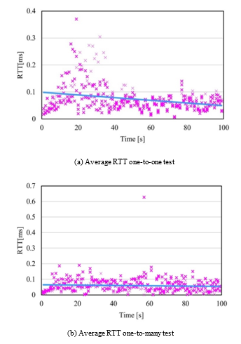Figure 12: Results average RTT

Table 1 shows a summary of the obtained results. From all the flows a total of 4.5Gbytes were transmitted in the 100s period, and the average of throughput was 96.6 Mbps with an average overall RTT of 0.07ms as expected since most of the lines were expedited.

• One-to-many Transmission Test

In this experiment, the continuous stream was sent from a single source to multiple destinations. In DSS, this case applies when a recovering a failed node or when reconstructing the data. To conduct this experiment, we sent an iperf request from H1 to a different TCP port in H5-H8 for 100s. A summary of the obtained results is described in Table 2. The discovered paths were {[a₁→b₁→ e→ h₁→ g₁] for H1, [a₃→c₁→ f→ i₁→ g₃] for H2, [a₄→c₂→ e→ h₃→ j₁] for H7, and [a₁→b₁→ f→ i₄→ j₄] for H8}, note that there is an overlap in the first segment of the paths which affected the overall throughput, as shown in Figure 11b, note the linear trend (in red) achieved 25% less than in the previous case. After tracing the costs of the paths, we found out that there were two paths with the same cost and the algorithm assigned the one first discovered,  which shared common segments. Nonetheless, the loss in throughput and the amount of data transferred (see Table 2) was compensated with a more homogeneous overall RTT, as seen in Figure 12b.

Table 1: Results Experiment 1 (one-to-one)

Flow#	Data [Gb]	AVG TP [Mbps]	AVG RTT[ms]
Flow 1	1.13	96.6	0.09
Flow 2	1.12	96.7	0.05
Flow 3	1.13	96.6	0.07
Flow 4	1.13	96.7	0.07

Table 2: Results Experiment 2 (one-to-many)

Flow#	Data [Gb]	AVG TP [Mbps]	AVG RTT[ms]
Flow 1	0.65	53.0	0.04
Flow 2	1.13	96.5	0.08
Flow 3	1.12	96.5	0.08
Flow 4	0.52	42.8	0.04

• Path Adaption Test

In this experiment, we test the resilience of the service by sending a continuous iperf request to a single server for 60s from H1 to H8, and after a random period, one of the links was shut down, Table 3 shows the results obtained. As observed, in the 60s a total of 624Mbytes were transmitted, with an average throughput of 85.6Mbps. Moreover, Figure 13 depicts the transmission trend, which was relatively stable. The initial path was calculated as follows a₁→b→e→h₄→j₂, then the link h₄→j₂ failed and recovered later on to a new path a₄→c→f→i₄→j₄, the outage time (shown in the red shaded part in the figure) was approximately 5s. Although the time could be reduced if only part of the path was modified, in practice it is more efficient to recalculate the whole path than look for the part that is affected as the time to add a flow is much lower than when it is updated [26]. Moreover, since the other flows will not have activity anymore, they will be removed in the next refresh cycle.

4.3.  Transmission with Background Traffic

In this section, we compare the approach with existing related work. Figure 14 shows the evaluation environment, which consists of a k-ary Fat-tree topology with K=4 pods. Eight servers (Pod 3 and Pod 4) will provide four storages represented as TCP ports. Without losing generality, for testing purposes, all of the links were configured to 100Mbps with a max_queue_size of 1000. Note that the topology was not augmented for this test, as the traditional techniques and the existing solutions could not handle the increased amount of redundancy, as the percentage of loss and drop packets was high. However, in the comparison, we also include the results in the case where the topology was augmented.

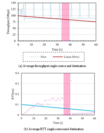Figure 13: Results path adaption test

Table 3: Results Experiment 3 (one-to-many)

Flow#	Data [Mbytes]	AVG Throughput [Mbps]	AVG RTT [ms]
Flow 1	624	85.7	0.06

To benchmark the approach, we compared the results with the following:

• Single path; the deployment was entirely handled by the L2Switch project in ODL, which uses the STP protocol and Dijkstra’s algorithm to calculate the shortest path for full connectivity.
• ECMP; An implementation of ECMP using a modified version of a publicly available code[4], that uses OF group rules to switch traffic when there are multiple paths.

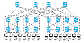Figure 14: Evaluation testbed 4-ary Fat-tree topology

• MPSDN [17]; the code is also publicly available[5], both the controller (Ryu[6]) and the mininet were hosted in the same virtual machine using Ubuntu 14.04 LTS (as the modified version of OVS was initially designed for a particular version of the kernel). We selected this work, as they proved that for certain conditions their performance equals the one of MPTCP, and thus, we implicitly benchmark our approach against this experimental protocol as well.
• Our approach; The deployment for our approach without modifying the topology, which means that no extra links were setup between the edge and aggregation layer in the topology. Moreover, the initial paths remained the same for the entire transmission, with no adaption.
• Extended version of our approach; For the extended version of the proposed approach, we modified the original Three-layer non-blocking FTN by adding an extra parallel link from the edge to the aggregation layer, and the paths were adapted after every 10s (refresh cycle) based on the information given by the Network Statistics

In the benchmark test, each host in Pod 3 and Pod 4 were listening to TCP ports {6001, 6002, 6003, and 6004}. Moreover, random UDP background traffic continuously sent from all host in Pod 1 and Pod 2 to all hosts in pods 3 and 4, i.e., H1 to H9, H2 to H10, H3 to H11 and so forth. We used continuous UDP iperf requests with bandwidths ranging from 1 to 10Mbps using the default paths and values. Then a request consisting of four parallel 100Mbps TCP iperf of were sent from both H1 and H5 (recovery nodes) which will be handled by the servers in Pod 3 and Pod 4 respectively. Therefore, the total amount of data sent was

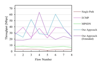Figure 16: Average throughput per flow

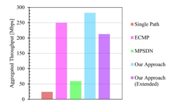Figure 17: Aggregated throughput at eight 100Mbps flows

800Mbps, and we measured the time in which all the transmissions finished.

• Completion time

The first metric we measured was the completion time. The results are depicted in Figure 15; as can be seen, the slowest solution was the single path approach, which completed all the data transferences in 275 seconds with a standard deviation of 16s. By contrast, the fastest one was the proposed approach in both of the cases, with and without topology augmentation, completing all the transference in a total of 30s with a standard deviation of 7.8s. In the case of the extended version of the proposal, the standard deviation was only of 4.8s which is the lowest among the benchmarked solutions. Note that ECMP completion time is also relatively low, 36.5s was the completion time of the last flow with a standard deviation of 6.4s. Finally, note that although MPSDN had a long completion time, 114s for the last flow, the variation of flow arrival was slightly higher than ours, which is due to the condition they use to ensure paths with compatible delays.

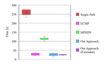Figure 15: Completion time of 800Mbytes in a 4-ary FTN

• Throughput

The second metric we measured was the average throughput per flow. As shown in Figure 16, MPSDN and the simple path approach showed a steady average throughput in all the flows. However, the overall maximum performance was low, which affected the completion time. In the other cases, even though the distribution was not as regular, the overall performance was much higher. Also, it is also worth noting that since the UDP traffic was sent at random bandwidths, some of the paths were more saturated than others, which might have caused the irregular distribution. Nevertheless, as can be seen in Figure 17, in our approach, the aggregated throughput was much higher than the other approaches. In the case of the augmented version, consider that although the number of links was duplicated from the edge to the aggregation layer, the increase was not linear.

• Network Load

The last variable we measured was the overall network load. Although the proposed approach can handle the dynamic load balance of servers and network at the same time as shown in [25], since the existing solutions focus mainly on the network load balancing we measured only that parameter. To perform this calculation, we used Tang’s [9] formula to calculate the network bandwidth utilization ratio , which gives the total bandwidth utilization in a time t and is expressed as in (3)

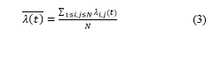Where N is the number of links, and λ_i,j is the link bandwidth utilization ratio defined as in (4), where b_i,j is the used bandwidth and B_i,j is the capacity of the link.

To make a fair comparison, we only measured the time until the time the first flow finished, which was about 30s from the beginning of the experiment. Figure 18 shows the Normalized the Cumulative Load over those 30s. As observed, ECMP was the solution that generated the most load over that time and across the whole network. However, the proposed approach used slightly more than the load of the single path solution with the added value of having a faster completion time and better overall throughput. Note that in our case, the load was not concentrated in a specific part of the network as in the other solutions, but spread among the discovered paths. Moreover, the results for the augmented version of the topology shows better traffic distribution, which will allow more concurrent operations to be performed in less time, a condition that is desirable for DSS.

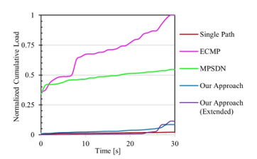Figure 18: Normalized Cumulative Network Load in 30s

Finally, Table 4 shows a summary of the results per flow. As observed, the proposed approach outperformed the others in most of the cases. Moreover, the overall load of the entire network is compared to the one on a single path, but the traffic is more evenly distributed. Note that the network load in ECMP and MPSDN per flow is relatively high, in the case of MPSDN, it might be due to the high amount of control messages sent by the controller, but in the case of ECMP, the use of multiple paths caused several retransmissions due to packet loss.

Table 4: Average benchmark results per flow

Metric	Single Path	ECMP	MPSDN	Our App.	Our App. (extended)
Completion Time [s]	256.5	27.5	113.6	26	24.4
Throughput [Mbps]	3.02	31.24	7.41	35.28	26.61
Network Utilization [%]	0.05%	2.06%	1.45%	0.11%	0.05%

5. Conclusions

Due to the restrictiveness of using legacy network techniques for DSS, it may not be possible to cope with the ever-increasing user content-generation in the future. Therefore, in this paper, we presented a network control method to improve DSS performance by using SDN. The proposed approach used pragmatic and straightforward solutions to handle DSS’s main requirements, namely aggregated bandwidth and effective use of resources. We have evaluated the proposal in various scenarios, and compared it with both network legacy techniques and existing solutions. Experimental results show that our method could achieve faster data transference and maintain balanced network and server loads. Additionally, in contrast to other proposals, our method does not require protocol or end-point modification but instead a topology enhancement based on the system demands. We showed that the overall performance of routinely DSS tasks can be dramatically increase by augmenting the DCN using parallel links, a proper path discovery, and dynamic adaption based on the network and servers load. As a future work, we still have to test the solution in large-scale and real DSS deployments. Furthermore, with the rise of new multipath transport protocols, such as QUIC [27] it might be interesting to study the impact on the way traffic is handled in non-traditional transport protocols in future networks. Likewise, we have not fully exploited the adaptive aspect of the proposal, which can be used to solve problems concerning resilient and fail-tolerant networks. Finally, it is also important to find a mechanism that achieves a tradeoff between high-performance and energy-efficiency of the whole network to cope with the proposed overprovisioned infrastructure.

Conflict of Interest

The authors declare no conflict of interest.

1.  L. Guillen, S. Izumi, T. Abe, T. Suganuma, H. Muraoka, “SDN im-plementation of multipath discovery to improve network perfor-mance in distributed storage systems” in 13th International Confer-ence on Network and Service Management, Japan, 2017. https://doi.org/10.23919/CNSM.2017.8256054
2.  D. Reinsel, J. Gantz, J. Rydning, “Data Age 2025: The evolution of data to life-critical – Don’t focus on big data; focus on the data that’s big”, IDC White Paper, 1–25, 2017.
3.  A. Dimakis, P. Godfrey, Y. Wu, M. Wainwright, K. Ramchandran, “Network coding for distributed storage systems” IEEE Transactions on Information Theory, 56(9), 4539–4551. 2010. https://doi.org/10.1109/TIT.2010.2054295
4. C. Suh, K. Ramchandran, “Exact-Repair MDS Code Construction Using Interference Alignment” in IEEE Transactions on Information Theory, 57(3), 1425–1442, 2011. https://doi.org/10.1109/TIT.2011.2105003
5.  N. B. Shah, K. V. Rashmi, P. V. Kumar, K. Ramchandran, “Distribut-ed storage codes with repair-by-transfer and nonachievability of inte-rior points on the storage-bandwidth Tradeoff” in IEEE Transactions on Information Theory, 58(3), 1837–1852, 2012. https://doi.org/10.1109/TIT.2011.2173792
6.  Open Networking Foundation (ONF) Software-Defined Networking (SDN) Definition Available at https://www.opennetworking.org/sdn-definition/ Accessed on 2018-07-20
7.  S. Kaneko, T. Nakamura, H. Kamei, and H. Muraoka, “A Guideline for Data Placement in Heterogeneous Distributed Storage Systems” in 5th International Congress on Advanced Applied Informatics, Ku-mamoto Japan, 942–945, 2016. https://doi.org/10.1109/IIAI-AAI.2016.162
8.  IEEE Std. 802.3ad “IEEE Standard for Local and metropolitan area networks – Link Aggregation,” available at http://www.ieee802.org/3/ad/ Accessed on 2018-06-10
9.  F. Tang, L. Yang, C. Tang, J. Li, M. Guo, “A Dynamical and Load-Balanced Flow Scheduling Approach for Big Data Centers in Clouds” IEEE Transactions on Cloud Computing, 2016. https://doi.org/10.1109/TCC.2016.2543722
10.  IETF RFC2992 “Analysis of an Equal-Cost Multi-Path Algorithm” available at https://tools.ietf.org/html/rfc2992, Accessed on 2018-01-30
11.  L. Li, Q. Xu, “Load Balancing Researches in SDN: A Survey,” in 7th IEEE Int. Conference on Electronics Information and Emergency Communication, 403–408, Macau China, 2017. https://doi.org/10.1109/ICEIEC.2017.8076592
12.  M. Al-Fares, S. Radhakrishnan, B. Raghavan, N. Huang, A. Vahdat, “Hedera: Dynamic flow scheduling for data center networks,” In 7th Conference on Networked Systems Design and Implementation, 19–34, San Jose CA USA, 2010. http://dl.acm.org/citation.cfm?id=1855711.1855730
13.  R. van der Pol, M. Bredel, A. Barczyk, B. Overeinder, N. van Adrichem, O. Kuipers, “Experiences with MPTCP in an Interconti-nental OpenFlow Network,” In 29th Trans European Research and Education Networking Conference,1–8, Amsterdam The Netherlands, 2013.
14.  IETF RFC 6182 “Architectural Guidelines for Multipath TCP Devel-opment,” available at https://datatracker.ietf.org/doc/rfc6182/, Ac-cessed on 2017-06-15
15.  J.P. Sheu, L. Liu, R.B. Jagadeesha, Y. Chang, “An Efficient Multipath Routing Algorithm for Multipath TCP in Software-Defined Net-works,” in European Conference Networks and Communications, 1–6, Athens Greece, 2016. https://doi.org/10.1109/EuCNC.2016.7561065
16.  D. J. Kalpana, K. Kataoka, “SFO: SubFlow Optimizer for MPTCP in SDN,” in 26th Int. Telecommunication Networks and Applications Conference, Dunedin New Zealand, 2016. https://doi.org/10.1109/ATNAC.2016.7878804
17.  D. Banfi, O. Mehani, G. Jourjon, L. Schwaighofer, R. Holz, “End-point-transparent Multipath Transport with Software-defined Net-works,” in IEEE 41st Conference on Local Computer Networks, 307-315, Dubai UAE, 2016. https://doi.org/10.1109/LCN.2016.29
18.  F. Carpio, A. Engelmann, A. Jukan, “DiffFlow: Differentiating Short and Long Flows for Load Balancing in Data Center Networks,” in IEEE Global Communications Conference, 1–6, Washington DC USA, 2016. https://doi.org/10.1109/GLOCOM.2016.7841733
19.  Y. Li, D. Pan, “OpenFlow based Load Balancing for Fat-Tree Net-works with Multipath Support,” In 12th IEEE International Confer-ence on Communications, Budapest Hungary, 2013.
20.  S. Izumi, M. Hata , H. Takahira, M. Soylu, A. Edo,T. Abe and T. Suganuma, “A Proposal of SDN Based Disaster-Aware Smart Routing for Highly-available Information Storage Systems and Its Evalua-tion,” International Journal of Software Science and Computational Intelligence, 9(1), 68–82, 2017. https://doi.org/10.4018/IJSSCI.2017010105
21.  K.T. Dinh, S. Kuklinski, W. Kujawa, M. Ulaski, “MSDN-TE: Multi-path Based Traffic Engineering for SDN,” in 8th Asian Conference on Intelligent Information and Database Systems, 630–639, Da Nang, Vietnam 2016. https://doi.org/10.1007/978-3-662-49390-8_61
22. P.H. Fredette, “The past, present, and future of inverse multiplexing,” in IEEE Com. Magazine, 32(4), 42–46, 1994. https://doi.org/10.1109/35.275334
23.  R. Toghraee, Learning OpenDaylight – The Art of Deploying Success-ful Networks, Packt Publishing Ltd., 2017.
24.  J. W. Suurballe, R. E. Tarjan “A quick method for finding shortest pairs of disjoint paths,” in Networks, 14(2), 325–336, 1984. https://doi.org/10.1002/net.3230140209
25.  L. Guillen, S. Izumi, T. Abe, T. Suganuma, H. Muraoka “SDN-based hybrid server and link load balancing in multipath distributed storage systems” in 2018 IEEE/IFIP Network Operations and Management Symposium, Taipei Taiwan, 2018. https://doi.org/10.1109/NOMS.2018.8406286
26.  M. Kuźniar, P. Perešíni, D Kostić “What You Need to Know About SDN Flow Tables,” in: Mirkovic J., Liu Y. (eds) Passive and Active Measurement. PAM 2015. Lecture Notes in Computer Science, 347–359, 2015. https://doi.org/10.1007/978-3-319-15509-8_26
27.  A. Langley, A. Riddoch, A. Wilk, A. Vicente, C. Krasic, et al “The QUIC Transport Protocol: Design and Internet-Scale Deployment.” in Proc. of the ACM Conference of Special Interest Group on Data Communication, 183–196, New York USA, 2017. https://doi.org/10.1145/3098822.3098842

(Click Here)

(Click Here)