1. Introduction

Co-variance analysis permeates almost all of system theory [1]. Based on the co-variance analysis, the probabilistic properties among random signals can be described. Naturally, the associate co-variance control problem became one of the most significant research topics for multi-variable stochastic systems. Since the system identification, Kalman filtering, stochastic distribution control and fault diagnosis are widely used in practice, the co-variance estimation and control are significant to all of these research areas and applications [2, 3, 4, 5]. In addition, the co-variance is also an ideal tool to analyze the performance of the stochastic systems for the probabilistic decoupling analysis [6, 7] and neural interaction analysis [8, 9].

During the past two decades, the main result of co-variance control is based on the Lyapunov equation while several conditions and controllers have proposed the control design for the co-variance assignment using the determined control signals [10, 11]. However, this controller is designed by Lyapunov equation without closed-form formulation. Since the closed-form model of state co-variance [12] presented in 2007, reduced order co-variance model [13] has been presented based on eigen-decomposition to solve output co-variance assignment (OCA) problem while the co-variance model was presented for the stochastic system with parametric uncertainty. However, all the existing results did not consider the control design with parametric uncertainties of the stochastic systems. Considering the uncertainties of the parameters, the robust controller has been designed in [14, 15, 16]. All the mentioned controllers can achieve good performance, however these methods have not been used to deal with the covariance analysis. To the best of our best knowledge, there is no existing solution to the parametric output feedback co-variance assignment for stochastic uncertain systems with the stability analysis. Therefore, it is significant to develop a simply output co-variance assignment (OCA) control law for the implementation of the complex dynamic multi-variable stochastic system with uncertainties.

In this paper, the stochastic uncertain multivariable systems have been investigated while the covariance assignment is very difficult since the uncertainties would affect the stability of the closed-loop systems. Based upon the investigated uncertain multivariable model, the transformed co-variance model can be obtained firstly, and then the controller and linear observer can be designed and analyzed. In particular, the sufficient conditions are given for the convergence of the observer, the stabilization of the controller and stabilization of the closed-loop system, respectively. In the end, the control input can be obtained by reversing the transformation. Using this control strategy, the design procedure is also given. Furthermore, the parameters of the controller and observer can be optimized using the parametric state feedback [17, 18] and entropy-based performance criterion. Using the presented control strategy, the optimal output feedback control law is obtained for OCA and the performance has been verified by the numerical simulation.

The rest of the paper is organized as follows. In Section 2, the formulation is given including the model formulation, transformed co-variance model and control objective. The parametric control strategy is developed while the convergence of the linear observer, the stabilization of the parametric state feedback controller and the stabilization of closed-loop uncertain system are analyzed in Section 3. Moreover, the parameter optimization and design procedure are also given in this section. Section 4 and Section 5 present the results of numerical simulation and the conclusions, respectively.

2. Formulation

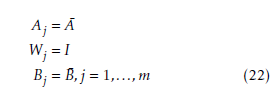
Suppose that the complex industrial dynamic process can be modeled by the following stochastic uncertain multi-variable system.

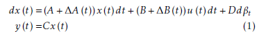where x ∈ _Rⁿ , u ∈ _R^s and y ∈ _R^m are the system state vector, input vector and output vector, respectively. β_t is the p-dimensional Wiener process. m, n and s are positive integers while system matrices A, B, C D and parameter uncertainties ∆A(t), ∆B(t) are of appropriate dimensions.

Notice that the model (1) can be rewritten as follows:

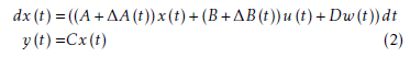where w is a standard Gaussian white noise. Without loss of generality, assume that the investigated system model (1) satisfies the following assumptions.

Assumption A1: Assume that the Gaussian noise vector w(t) satisfies

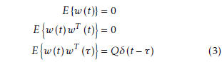where δ(·) is the Dirac delta function.

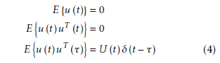
Assumption A2: Similar to the assumption of the noise, assume that the control signal is restricted by

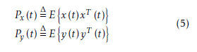
Based on the definition of the co-variance matrix, the state and output co-variance matrices of the given system are given by

In addition, the co-variance matrices can be rewritten as follows:

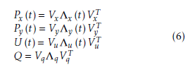where Λ_x, Λ_y, Λ_u and Λ_q are real diagonal matrices. V_x, V_y, V_u and V_q are associated orthogonal matrices. All of the matrices are with the same dimensions as the associated vectors.

Therefore, the reduced-order closed-form covariance model can be obtained following the vectorization operation.

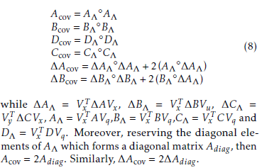
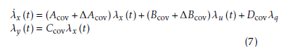where λ_x, λ_y, λ_u and λ_q are the diagonal elements of matrices Λ_x, Λ_y, Λ_u and Λ_q, respectively. The coefficient matrices can be calculated using Hadamard product as follows:

Thus, the control objective is to develop a new control strategy to assign the state of the transformed model (7) so that the covariances and variances of the system outputs can be assigned simultaneously.

To achieve the mentioned control objective, the following assumption should be taken into account:

Assumption A3: The pair (A_cov,B_cov) is controllable.

Assumption A4: The admissible parameter uncertainties are of the norm-bounded form

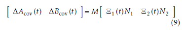In Eq. (9), M, N₁ and N₂ denote the structure of the uncertainties which are known real constant matrices with proper dimensions. Ξ₁(t) and Ξ₂(t) are unknown time-varying matrices which respectively meet the following conditions.

In addition, the following lemma [19] has been recalled here which can be used to analyze the convergence and stabilization of the presented control strategy.

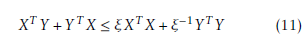
Lemma 1. Given any real constant matrices X and Y with proper dimensions. Then there exists a constant ξ > 0, such that the following inequality holds.

3. Control Strategy

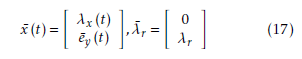
The reference co-variance matrix can be rewritten as follows:

Since the diagonal matrix r can be arranged as vector λ_r, the co-variance assignment problem transfers to state tracking problem using the presented reducedorder co-variance model if we set V_y = V_r.

To track the desired state co-variance vector, the integrator should be considered in the control scheme. The error vector e_y (t) = λ_rλ_y is treated as the extended state and substitutes the error into the closed-loop system.

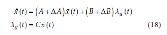
Then, the closed-loop system in the state-space form can be obtained as follows:

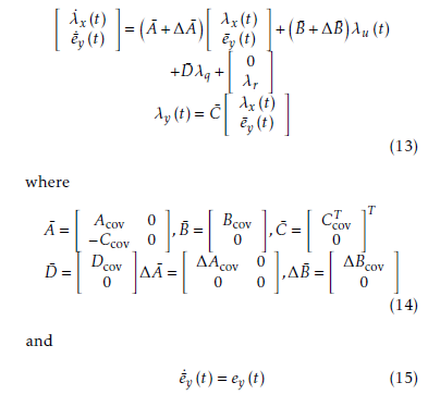We can further present the closed-loop system in compact format as follows:

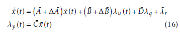
Notice that Dλ¯ _q and λ¯_r are real constants which means that if the following system is stabilized then the variance and co-variance assignment can be completed.

Based upon the transformed system model 18, the control strategy can be divided into two parts: observerbased output feedback design and the parametric optimization for uncertainty compensation.

3.1. State feedback design

The linear state feedback controller can be determined by the nominal linear model and the control law is described by

where the gain matrix K can be obtained by parametric design [17, 13]. In particular, we have

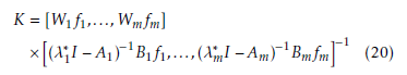where modified parameter vectors and closed-loop eigenvalues are denoted by f₁,…,f_m and ,…,λ^∗_m which can be considered as free parameters. In the case of a common open-loop and closed-loop eigenvalue, the gain matrix K can be determined by the following equations.

where v_j⁰ and w_j⁰ denote the open-loop eigenvectors and eigenrows of A_j. b_i is the i-th column of B¯. e_i is a unit vector while the i-th element is 1. In the other case, no common eigenvalue results in w_j^0T b_i = 0 which leads to

Substituting control law (19) into the transformed system model (18) yields the closed-loop system:

where A_c = A¯+BK¯ , ∆A_c (t) = ∆A¯(t)+∆B¯(t)K. Thus the following lemma can be proposed.

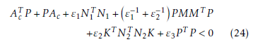
Lemma 2. For the uncertain multi-variable system given by (18), with the assumptions and with the control law given by (19), then there exist two positive constants ε₁ and ε₂, so that the equilibrium x¯(t) = 0 is stabilized if the following matrix inequality has a positive-definite solution

Proof. Consider the Lyapunov function candidate as

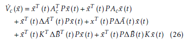
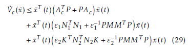
The time derivative of V_c (x¯) along the trajectories of (23) is given as follows.

Let ε₁ and ε₂ be positive constants, the following matrix inequalities hold using Lemma 1.

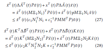Substituting these inequalities into the derivative of V_c (x¯) with Assumption 4, we have

Since V˙_c (x¯) < 0 , the proof of lemma 2 is completed.

3.2. Observer design

Using the linear observer to estimate the states of the model (18), the linear observer can be designed based on the nominal linear model.

where the estimated vector can be denoted by x¯ˆ and L is pre-specified gain matrix of this observer.

Introducing the error of the estimation by

and substituting the Eq. (30)-(31) to system model (18). The closed-loop model can be described by

where A_o = A¯ − LC¯. Similar to Lemma 2, Lemma 3 is given as follows.

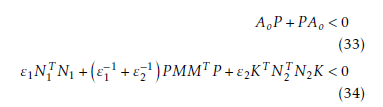
Lemma 3. For the uncertain multi-variable system given by (18), with the assumptions and with the linear observer given by (30), then there exists two positive constants ε₁ and ε₂, so that the estimation error e(t) converges to zero if the following matrix inequalities have a positive-definite solution P = P ^T > 0.

Proof. Consider the Lyapunov function candidate as

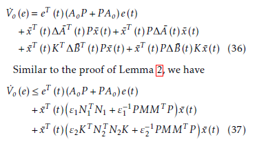
The time derivative of V_o (e) along the trajectories of (31) is given by the following equation.

which ends the proof

3.3. Output feedback design

Combining the parametric state feedback controller and the designed observer, the output feedback controller can be obtained for the system (18).

which leads to the closed-loop dynamics as follows.

Furthermore, the stability of the closed-loop control design can be guaranteed by the following theorem.

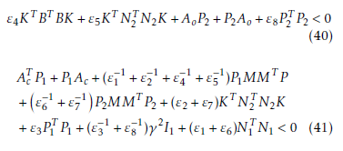
Theorem 4. For the uncertain multi-variable system given by (18), with the assumptions and with the control law given by (38) using the observer (30), then there exists two sets of positive constants ε_i,i = 1,…,2 and ε_j,j = 4,…,7, so that the equilibrium x¯(t) = 0 is stabilized if the following matrix inequalities have positive-definite solution P₁ = P₁^T > 0,P₂ = P₂^T > 0.

Proof. Consider the Lyapunov function candidate as

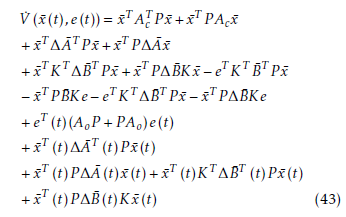
The time derivative of V (x¯(t),e(t)) along the trajectories of (39) is shown as follows.

Let ε₄ and ε₅ be positive constants, the following matrix inequalities hold using Lemma 1.

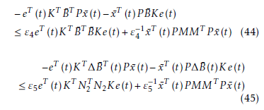Substituting these inequalities into the derivative of V (x¯(t),e(t)) and using Lemma 3, we have

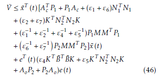which leads to the conditions and the proof has been completed.

3.4. Parametric optimization

Notice that all the free parameters can be adjusted without changing the stability of the system, which means that the optimization of the parameters can be done for various performance criteria. In this paper, we design the controller based on the nominal model then the optimization can be considered as the uncertainty compensation using the following performance criterion.

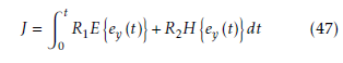where real positive R₁ and R₂ stand for the weights. H {·} denotes the entropy. To simplify the performance criterion, the entropy can further be replaced equivalently by information potential [20, 21].

Then the optimal free parameter f_i can be obtained by gradient descent once the eigenvalues λ^∗_i are prespecified.

where j denotes the optimization searching iteration index. µ stands for the pre-specified step.

Once the control law λ_u is obtained, the control input u(t) for system (1) can be calculated by reversing the transformation. In particular, Λ_U can be obtained by λ_u and we have

where ξ (t) denotes the standard Gaussian white noise.

Remark 1. The actual control law is non-linear though the transformed system model is linear.

Remark 2. Based on the dual principle, the observer gain matrix can be also obtained using proposed optimization approach. Meanwhile, the optimization operation can also be replaced by multi-objective optimization algorithms then the weights can be neglected.

Remark 3. Only a few elements of the parameter vectors f_i affect the control performance directly. Therefore, in order to determine the free parameters quickly, trial and error method can be used and the performance criterion can verify the manually selected parameters simply.

3.5. Design procedure

The procedure of the proposed control strategy is summarized as follows:

Step1 Transfer the system to co-variance assignment model.

Step2 Setup the initial free parameters of the controller.

Step3 Use the numerical approach to optimize the performance criterion (47), by computing the mean, the entropy and gradient descent, then the optimal parameters are obtained.

Step4 Update the feedback gain matrix of the control law (19, 49), and verify it by the conditions of Lemma 2 to guarantee stability of the system, if the conditions hold, then go to next step, otherwise, return to Step 1.

Step5 Obtain the feedback gain matrix of the observer by dual principle and verify it by Lemma 3.

Step6 Verify the optimal parameters by Theorem 4, and if the conditions can be satisfied, then complete the procedure, otherwise, return to Step 2.

Step7 reverse the transformation and obtain the control input by (49).

4. A Numerical Simulation

To verify this new model and the control algorithms proposed in this paper, one numerical example is presented in this section.

The original model can be shown as below: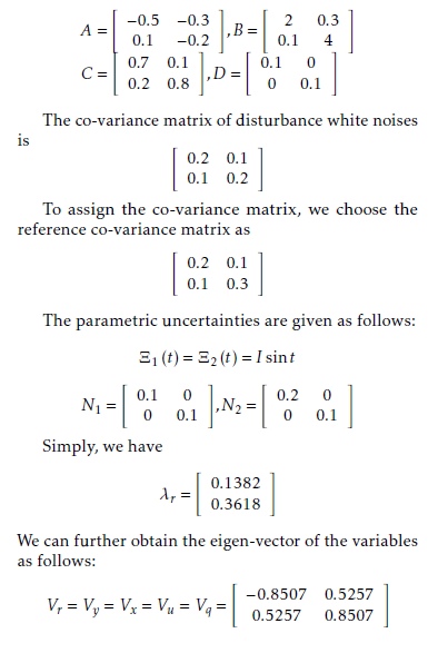

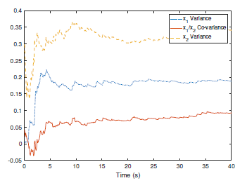Figure 1. The measured co-variance and variances of the system outputs.

Following the presented control strategy, the simulation results have been shown by Fig. 1-4. Particularly, Fig. 1 indicates the co-variance and variances of the system outputs. Comparing to the reference covariance matrix, the practical system outputs achieve the assignment with uncertainties. Meanwhile, Fig. 2 shows that the system outputs are stable if the transformed co-variance system design is stabilized while the states and control inputs of the transformed co-variance model have been given by Fig. 3 and Fig. 4. It has been shown that the eigenvalues of the co-variance matrix are tracking the reference eigenvalues of the reference co-variance matrix and the practical control input can be obtained by reversing the transformation using the values of the designed control input of the transformed co-variance model.

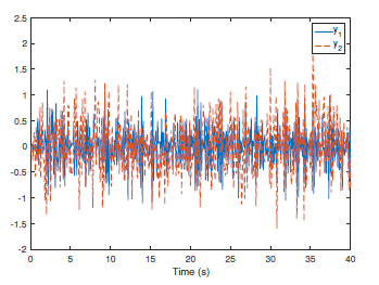Figure 2. The outputs of the system.

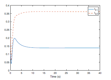Figure 3. The state assignment of the transformed covariance model.

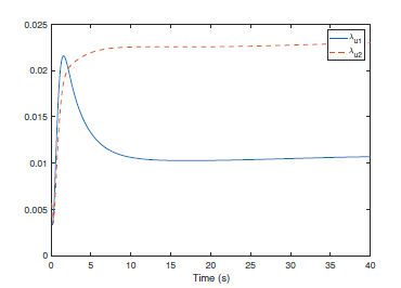Figure 4. The designed control input of the transformed co-variance model.

5. Conclusion

This paper investigates the co-variance assignment strategy for a class of multi-variable stochastic uncertain systems. Combining the reduced-order covariance model and parametric feedback, the control strategy is obtained by output feedback stabilization. In particular, the transformed model is given firstly with the extended co-variance assignment error. Then the linear observer is designed to estimated the extended state of the transformed model. After that, the output feedback is obtained via parametric optimization. Meanwhile the theoretical analysis is given to guarantee the robustness, stabilization and convergence of the closed-loop systems. Based on the results of the numerical simulation, the effectiveness of the presented control strategy has been verified while the control objectives have been achieved. Since the covariance assignment is widely used in practical systems, such as paper-making process, the industrial applications using the presented control strategy will be the potential extension as a future work.

Conflict of Interest

The authors declare no conflict of interest.

Acknowledgement

The authors would like to thank the anonymous reviewers for their valuable comments.

1.  A. Hotz and R. E. Skelton, “Covariance control theory,” International Journal of Control, vol. 46, no. 1, pp. 13–32, 1987.
2.  K. Liu, K. Li, and C. Zhang, “Constrained generalized predictive control of battery charging process based on a coupled thermoelectric model,” Journal of Power Sources, vol. 347, pp. 145–158, 2017.
3.  M. Ren, J. Zhang, M. Jiang, M. Yu, and J. Xu, “Minimum (hphi)– entropy control for non-gaussian stochastic networked control systems and its application to a networked dc motor control system,” IEEE Transactions on Control Systems Technology, vol. 23, no. 1, pp. 406–411, 2015.
4.  L. Guo, L. Yin, H. Wang, and T. Chai, “Entropy optimization filtering for fault isolation of nonlinear non-gaussian stochastic systems,” IEEE Transactions on Automatic Control, vol. 54, no. 4, pp. 804–810, 2009.
5.  L. Yao, J. Qin, H. Wang, and B. Jiang, “Design of new fault diagnosis and fault tolerant control scheme for non-gaussian singular stochastic distribution systems,” Automatica, vol. 48, no. 9, pp. 2305–2313, 2012.
6. Q. Zhang, J. Zhou, H. Wang, and T. Chai, “Minimized coupling in probability sense for a class of multivariate dynamic stochastic control systems,” in Decision and Control (CDC), 2015 IEEE 54th Annual Conference on. IEEE, 2015, pp. 1846–1851.
7.  “Output feedback stabilization for a class of multivariable bilinear stochastic systems with stochastic coupling attenuation,” IEEE Transactions on Automatic Control, vol. 62, no. 6, pp. 2936–2942, 2017.
8. Q. Zhang and F. Sepulveda, “A statistical description of pairwise interaction between nerve fibres?” in Neural Engineering (NER), 2017 8th International IEEE/EMBS Conference on. IEEE, 2017, pp. 194–198.
9.  “A model study of the neural interaction via mutual coupling factor identification,” in Engineering in Medicine and Biology Society (EMBC), 2017 39th Annual International Conference of the IEEE. IEEE, 2017, pp. 3329–3332.
10.  K. Yasuda and R. E. Skelton, “Covariance controllers: A new parameterization of the class of all stabilizing controllers,” in American Control Conference, 1990. IEEE, 1990, pp. 824–829.
11.  K. M. Grigoriadis and R. E. Skelton, “Minimum-energy covariance controllers,” Automatica, vol. 33, no. 4, pp. 569–578, 1997.
12.  H. Khaloozadeh and S. Baromand, “State covariance assignment problem,” IET control theory & applications, vol. 4, no. 3, pp. 391–402, 2010.
13.  Q. Zhang, Z. Wang, and H. Wang, “Parametric covariance assignment using a reduced-order closed-form covariance model,” Systems Science & Control Engineering, vol. 4, no. 1, pp. 78–86, 2016.
14.  Z. Wang, B. Huang, and H. Unbehauen, “Robust reliable control for a class of uncertain nonlinear state-delayed systems,” Automatica, vol. 35, no. 5, pp. 955–963, 1999.
15.  T. Shen and K. Tamura, “Robust h/sub/spl infin//control of uncertain nonlinear system via state feedback,” IEEE Transactions on Automatic Control, vol. 40, no. 4, pp. 766–768, 1995.
16.  Q. Zhang and X. Yin, “Observer-based parametric decoupling controller design for a class of multi-variable non-linear uncertain systems,” Systems Science & Control Engineering, vol. 6, no. 1, pp. 258–267, 2018.
17.  G. Roppenecker, “On parametric state feedback design,” International Journal of Control, vol. 43, no. 3, pp. 793–804, 1986.
18. G. Roppenecker and J. O’reilly, “Parametric output feedback controller design,” Automatica, vol. 25, no. 2, pp. 259–265, 1989.
19.  I. R. Petersen, “A stabilization algorithm for a class of uncertain linear systems,” Systems & Control Letters, vol. 8, no. 4, pp. 351–357, 1987.
20.  Q. Zhang and A.Wang, “Decoupling control in statistical sense: minimised mutual information algorithm,” International Journal of Advanced Mechatronic Systems, vol. 7, no. 2, pp. 61–70, 2016.
21.  Y. Zhou, Q. Zhang, H. Wang, P. Zhou, and T. Chai, “Ekf-based enhanced performance controller design for nonlinear stochastic systems,” IEEE Transactions on Automatic Control, vol. 63, no. 4, pp. 1155–1162, 2018.

(Click Here)

(Click Here)