1. Introduction

This paper is an extension of work originally presented at the Military Communications Conference [1]. Wireless sensor networks are a class of networks in which some or all of the sensors or resources collect, analyze, and communicate data acquired from their environment (external or internal) to other nodes in the network [2]. These other nodes could be resources, sensors, or fixed or mobile command posts. Mobile adhoc networks (MANETs) are a subset of wireless sensor networks that have an absence of a fixed infrastructure, and exhibit a dynamic communication topology [3]. Resources within transmission range of others communicate directly (depending on bandwidth limitations) and cooperation among intermediate resources is required for resources to communicate with others outside of their direct communication range. More and more networks, in both the military and commercial domain, are relying on wireless sensor networks and MANETs [4, 5, 6].

The ability for data to be collected by manned and unmanned vehicles engaged in military, government, and commercial missions is increasing at an exponential rate [7]. Examples include high-resolution video, telephone intercepts, traffic congestion reports, internal vehicle system states, among others. In commercial telecommunication networks, there are instances where the capacity across the network is in the terabytes per second range [8]. Networks of this type have the ability to transmit all data that is collected without restrictions or delays. However, in times of crisis and disaster, commercial and civil communication networks can be severely degraded [9, 10]. And in military missions, bandwidth is oftentimes severely limited, which results in a reduction in transmission and sharing of information that can be mission-critical. And this will continue to be the case due to the rise of operations performed in anti-access/area denial (A2AD) environments, against near-peer adversaries. In the past, this meant that information collected by vehicles would not be processed, analyzed, and understood until after the vehicle had returned to base and ‘uploaded’ all of the collections [7, 11].

In performing more of the processing and analysis on-board the vehicles, there has the potential for less bandwidth requirements for vehicles to share information important for mission success. In effect, this can be seen as pushing the smarts out to the tactical edge. Each generation of manned and unmanned vehicles is having more and more processing capabilities onboard [11]. Examples include internally monitoring on-board systems, fusing information collected from various on-board sensors, picking out a person of interest from a full motion video, and deciding how much information should be sent over the sensor network and to whom should be the recipient of such information [12]. While some of the collected information can just be generated and stored on a vehicle, and offloaded upon mission completion, other generated information is vital to mission success, and must be transmitted to control station(s) or other resources during mission execution.

To address this, we consider the following problem. There are a set of resources (moving or fixed) that have a set of Information Generation Requests (IGRs) to satisfy over a given time horizon. If a resource executes a task to perform the IGR, then an associated piece of information is generated. We will use the term IGR to denote the information that gets generated. Each IGR can come from one of a fixed set of categories (for an example of information categories, see Table 1). In addition, each IGR has associated with it the following characteristics: an expected time of generation, the set of consumer resources (those resources that would find this information important for their mission), the time by which the information needs to be delivered to the to be of use, the expected original size of the information, and the priority of the information (i.e., a measure of its importance in the mission). We note that the priority of an IGR could be determined a priori (e.g., information collected about one kinematic location is deemed very important and therefore is given a high priority) or dynamically on-board the resource at the time of collection, if the resource has the appropriate analytics (e.g., image is given low priority because it does not contain any red cars). By a ‘consumer resource’ for a particular IGR, we mean that the resource actually performs some processing with that information (e.g., fuses that information with other information [13, 14], makes command and control decisions, etc.).

There is a dynamic sensor network topology in place over the time horizon. This dynamic network has finite, but varying bandwidth limitations between any two resources at any given time, and in many cases there might not be a direct connection between two resources. Each IGR can be sent over the network with different potential granularities (e.g., 100% of original size, 70% of original size, etc.), but there is a minimum size percentage with which the information remains useful to the consumer of the information. As an IGR gets routed from the generating resource to the consumer resource, all resources along this route will need to store this IGR locally for some amount of time. The generating resource will need to store an IGR from the time of generation until the IGR is completely sent to the next resource in the path to the consumer resource(s). Non-consumer resources along this path will need to store the IGR from the time the resource begins receiving the IGR until the time the resource has completely transmitted the IGR to the next resource along the path. And the consumer resource(s) will need to store the IGR form the time they begin receiving it until at least they have finished processing the IGR.

Each resource has a finite storage capacity, and resources can triage information they have stored (e.g., once a piece of information is generated and completely sent to the next resource along the path to the consumer, the generator resource can delete the information from storage). The objective is then to determine which IGRs to route over the network, how to route those IGRs so that they have a minimal time delay (difference between time of consumption and time of generation), from generating resource to consumer resource over the time horizon, while also attempting to maximize the size of granularity of each IGR that is routed. In turn, this produces the higher-level end product of determining which IGRs should be accomplished for mission objectives, given the network topology characteristics.

There has been some prior research into routing schemes for collected data across a dynamic network. In [17], the author considered the problem of sinkholes in a network. A sinkhole node attempts to deceive all the nodes in the network to route network traffic to the sinkhole, by broadcasting false routing information across the network. An approach based upon secondary caching was developed to prevent a sinkhole attack in dynamic source routing sensor networks. In [18], the author consider cellular data networks and the significant increase in data being transmitted over these networks. Their research looked at data traffic management techniques, whereby users and automated approaches ‘flag’ messages that are of low priority, and an higher-level agent-based scheduling system had the ability to delay scheduling of low priority messages during peak load times. In [19], the authors considered the problem of extending lifetimes of wireless sensor networks. In their view, the sending of redundant data across sensor networks reduced the lifetime of these networks. They looked at providing certain nodes in the network to function as ‘data aggregation’ nodes, receiving collected data from other nodes in the network, fusing or aggregating the data together to reduce redundant information, and then passing this reduced set of data onwards to a base station. They employed a grid-based routing and aggregator selection scheme to find the minimum number of aggregation points while routing data to the base station ensuring that the network lifetime is maximized.

Table 1: Examples of Information Categories. Category Example Internal System State Measurements on the engine pressure ratio [15] External Collection Photographs of an urban traffic intersection Situation Assessments High likelihood that red truck contains person of interest Command and Control (C2) Modifying flight plan to conserve battery life [16]

In addition, there has been some prior research addressing certain aspects of our problem of interest, but none that has addressed the problem completely. In [20], the author considered the problem of routing information across a network, from a workflow perspective, but the network was assumed to be complete and static, and bandwidth was not addressed. In [21], the researchers extended this work to include bandwidth limitations, but still under the assumption on a complete and static network. In [22], the researchers presented a mixed-integer linear programming formulation to model the trajectory of a set of unmanned aerial vehicles, along with routing of information collected from these vehicles back to a base station. They did not consider bandwidth fluctuations in the sensor network, and the resources were not the recipient of any information, just the base station. In addition, all of their information was considered to have the same priority. In [23], the author considered underwater acoustic networks and the long propagation delays and low bandwidths inherent in such networks. A set of nodes was using the same bandwidth channel, and because their problem had bursty data, the solution approach looked at submitting their requests randomly, as demand dictated. A medium access control protocol was in place to minimize the number of collisions among the information flowing across the network. In [24], the researchers investigated ways to enhance the operations of a power grid. One of the ways, taking advantage of the high sampling rates of the measurement data, required a high bandwidth, networked communication system. Their results derived a method to simulate, design, and test the adequacy of a communication system for a particular grid layout.

The rest of this paper is organized as follows. In Section 2, we introduce the parameters and decision variables for our model, and rigorously derive the mathematical program representing our problem. Section 3 develops a heuristic to efficiently find good quality solutions. Section 4 analyzes the results of computational experiments performed on various scenarios, comparing commercial software solving a linearized version of the mathematical program and the solutions found by the heuristic. Section 5 provides some concluding remarks and future research directions.

2. Mathematical Formulation

In this section, we rigorously derive mathematical equations to model the problem of interest. This results in a mixed-integer nonlinear program (MINLP). We note that the time dimension in the model is discretized, over the planning horizon of K time-steps.

2.1.     Parameters

This section lists the parameters for the mathematical programming problem.

• is the set of resources, i,i₁,i₂,∈ I;
• is the number of Information Generation Requests (IGR)s, j ∈ {1,…,J };
• is the number of time-steps in the planning horizon, k,k^ˆ ∈ {1,…,K};

P ^min is the minimum percentage an IGR can be decreased in size and still be considered useful to consumer resource(s);

τ_i,j is the number of time-steps after a consumer receives an IGR before the consumer can delete the IGR, i.e., the number of time-steps it takes resource i (the consumer resource) to ‘process’ IGR j; ρ_j is the expected priority of IGR j; S_j^o is the expected original size of IGR j; g_j is the expected time of generation of IGR j;

d_j is the time by which IGR j is due to the consumer resource(s) of the IGR;

L_i is the storage capacity of resource i; b_i1,i₂,k is the expected bandwidth capacity from resource i₁ to resource i₂ at time-step k; ρ¯ is the largest expected priority, i.e., ρ¯ =

h i max ρ_j ; j

ω_d and ω_s are the weighting coefficients for the priority and size components of the objective function;

M is a large enough constant, used in Constraints

2.2. Variables

This section lists the decision variables for the mathematical programming problem.

s_j = the size of IGR j sent to the consumer resource(s), ∀j;

a_i1,i₂,j,k = the amount (size) of IGR j sent from resource i₁ to resource i₂ during time-step k, ∀i₁,i₂(, i₁),j,k;

m_i,j,k = the amount of IGR j being stored on resource i at time-step k, ∀i,j,k. N.B.: For consistency of the constraints, m_i,j,0 = 0 ∀i,j;

β_i,j = the amount of time resource i takes in sending IGR j to other resources, i.e., the time between resource i completely receiving or generating IGR j to the time where resource i no longer needs IGR j, ∀i,j;

T_i,j = the time-step at which resource i completely receives (or generates) IGR j, ∀i,j;

N.B.: For consistency of the constraints, it is necessary to set e_i,j,0 = 0 ∀i,j. Also, note that e_i,j,k = 1 implies that e<sub>i,j,`</sub> = 1 for each ` > k and e_i,j,k = 0 implies that e<sub>i,j,`</sub> = 0 for each ` < k.

2.3.  Nonlinear Mathematical Formulation

This section presents the mathematical model of the problem described in Section 1, resulting in a mixedinteger nonlinear program (MINLP).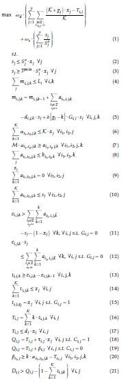

2.4 Interpretation of Nonlinear Mathematical Formulation

In this section, we explain the objective function and each of the constraints that are part of the mathematical formulation.

• The objective function, Equation (1), is a weighted combination of the time delay and size of the IGRs routed across the network.

The first term in the objective function deals with the time delay of those IGRs chosen to be routed. The sum is over all IGRs j and all resources i that are consumers of IGR j (i.e., those resources such that the parameter C_i,j = 1). When an IGR j is not chosen to be routed, x_j is set to be 0 and T_i,j also ends up as 0, so this term is 0. When an IGR is chosen to be routed, x_j is set to be 1 and T_i,j is set to be the time at which resource i completely receives IGR j. The time IGR j is generated is given by the parameter g_j. The maximum value of this term is 1, which occurs when T_i,j = g_j (which is an idealistic situation), while

K+g_j−d_j the minimum value of this term is _K , which can be 0 when g_j is 0 and d_j is K.

The second term of the objective function deals with the size of the IGRs chosen to be routed, looking at the ratio of the actual size of the IGR that gets routed versus the original size.

Note that that scale of these two terms are the same, i.e., they are both within [0,1], and are unit-less. The first term is weighted by ω_d, while the second term is weighted by ω_s.

• Constraints (2) force s_j to be less than or equal to S_j^o if IGR j is chosen to be routed, and 0 if IGR j is not chosen to be routed;
• Constraints (3) require s_j to be greater than or equal to the minimal amount to be routed for IGR j (P ^min S_j^o), if IGR j is chosen to be routed;
• Constraints (4) ensure that at each time-step, the storage capacity for each resource is not exceeded;
• Constraints (5) determine the amount of IGR j stored on resource i at time k as the amount stored at time k − 1 plus the amount sent to resource i at time-step k minus s_j if IGR j is deleted from resource i’s storage at time-step k, plus s_j if IGR j is chosen to be routed by resource i and is generated at time-step k. N.B.: The Dirac-Delta impulse function δ[q] returns 1 when q = 0 and returns 0 otherwise [25];
• Constraints (6) only allow α_i1,i₂,j,k to be greater than 0 if IGR j is chosen to be routed;
• Constraints (7) force a_i1,i₂,j,k to be 0 if resource i₁ is not sending IGR j to resource i₂ at time-step k;
• Constraints (8) limit the amount of information traveling from resource i₁ to i₂ at time-step k to be no more that the capacity of this edge, b_i1,i₂,k;
• Constraints (9) enforce that no resource can send IGR j before it is generated;
• Constraints (10) enforce that resource i₁ send no more than s_j of IGR j to resource i₂;
• For those resources that do not generate IGR j and IGR j is chosen to be routed, Constraints

(11) force e_i,j,k to be 1 if all s_j of IGR j reaches resource i at or before time-step k. This constraint allows e_i,j,k to be 0 or 1 otherwise;

• For those resources that do not generate IGR j, Constraints (12) force e_i,j,k to be 0 while not all s_j of IGR j has reached resource i. This constraint allows e_i,j,k to be 0 or 1 otherwise;
• Constraints (13) set t_i,j,k to be 1 at the time-step that resource i receives all s_j of IGR j, and to be

0 for all other time-steps;

• Constraints (14) enforce that resource i can receive IGR j at most once;
• Constraints (15) set t_i,j,k equal to 1 if IGR j is chosen to be routed, is generated by resource i, and k is the time of generation of IGR j;
• Constraints (16) set T_i,j to be the time at which resource i receives IGR j;
• Constraints (17) enforce that any resource that receives IGR j, must do so before its due date/time, if IGR j is chosen to be routed;
• Constraints (18) define the time at which resource i has completely ‘processed’ IGR j, if resource i is a consumer of IGR j and IGR j is chosen to be routed;
• Constraints (19) define the time at which resource i has completely transmitted IGR j to other resources, if resource i is not a consumer of IGR j and IGR j is chosen to be routed;
• Constraints (20) determine the amount of time it takes resource i to send IGR j to other resources, once resource i receives or generates IGR j;
• Constraints (21) ensure that if IGR j is chosen to be routed, that IGR j cannot be deleted from resource i until resource i is finished with the IGR;
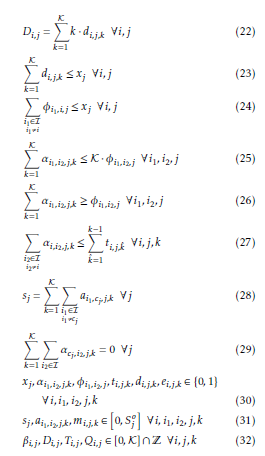
• Constraints (22) determine the time at which resource i deletes IGR j;
• Constraints (23) ensure that resource i can delete IGR j at most once;
• Constraints (24) enforce that at most one resource is assigned to send IGR j to resource i;
• Constraints (25) only allow resource i₁ to send IGR j to resource i₂ if it is assigned to;
• Constraints (26) force i₁ to send IGR j to resource i₂ during at least one time-step, if i₁ is assigned to send IGR j to resource i₂;
• Constraints (27) does not allow resource i to send any portion of IGR j at time-step k if resource i has not completely received (or generated) IGR j by time-step k − 1;
• Constraints (28) ensure that the consumer resource(s) of IGR j receives all s_j units, if IGR j is chosen to be routed;
• Constraints (29) prohibit resource c_j (the consumer of IGR j) from sending IGR j to other resources;
• Constraints (30) – (32) are domain restriction constraints on the decision variables.

3 Solution Methodologies

The formulation derived in Section 2.3 is a nonlinear mixed-integer programming problem. However, this formulation can be linearized through standard techniques from operations research [26], resulting in a mixed-integer linear program (MILP). As such, in theory the MILP formulation could be solved using a number of commercial software packages (e.g., CPLEX [27], LINDO [28], etc.). It can be shown that this optimization problem is NP-Hard, as a variant of the vehicle routing problem with split deliveries and time windows [29, 30, 31], which necessitate heuristic strategies for finding good-quality solutions efficiently [32, 33] when the problem instances are of sufficient size.

The heuristic developed is split into two phases, an Information Routing phase, and a Storage Management phase. The Information Routing phase attempts to route all of the IGRs, from generating resource to consuming resource(s), without consideration of storage limitations on the individual resources. The only constraints taken into account in the Information Routing phase are the bandwidth limitations across the sensor network. The Storage Management phase of the heuristic then factors in the storage limitations of each resource to reduce the solution to one that is feasible.

Figures 2 and 1 provide pseudo-code for the Information Routing and Storage Management phases, respectively. The Information Routing function is input the set of IGRs (and all information about the IGRs), the initial allocation of bandwidth across the network over time (InitCommBW), the minimum percentage (in size) an IGR is able to be reduced and still be useful (MinSizePercent), and the ratio by which to reduce the size of the IGR in sending over the network, if needed (GranularityRatio). Lines 1 to 5 initialize internal variables. Lines 6 to 32 get executed while there are still IGRs on the list to be routed. For each IGR still on the CurListIGRs list, lines 7 to 25 attempt to determine a route for the IGR that allows for at least the minimum size for the IGR to be routed. Line 8 computes the size of the current IGR and line 9 computes the minimal allowable size of the IGR to be routed. While a feasible route for the current IGR has not been found, and the current size of the IGR is larger then the minimum allowable size, lines 11 to 19 get executed. Line 11 calls the function ComputeRoute, given the current size of the IGR and the current allocation of bandwidth across the network. Returned from this function are the route for this IGR from generating resource to consumer resource, as well as the time the IGR will completely reach the consumer resource. If the time by which the consumer completely receives the IGR is less than the due date of the IGR, then a potential route for this IGR is found, and the potential time delay for this IGR is computed. Otherwise, the size of the IGR is reduced by the granularity ratio. If a potential route is not found in lines 11 to 19, then this IGR is moved to the NotRoutedIGRs list and removed from the current list of IGRs (lines 21 and 22). Line 23 also sets this IGR to have a delay time of +∞. After the code in lines 7 to 25 is completed, the heuristic greedily selects the IGR with the current minimal potential delay time (line 26). This IGR is removed from the list of current IGRs, and added to the list of routed IGRs. The potential route computed for this IGR is

procedure Storage Management(ResourceList, RoutedIGRs, NotRoutedIGRs, MaxStorageSize) 1                      CurrentRL ← ResourceList; 2                      while CurrentRL , ∅ do 3                      CurR ← Choose(CurrentRL); 4                      CurrentRL ← CurrentRL\CurR; 5                      for k = 0 to K do 6                      for each IGR` completely transited through CurR by time-step k do 7                      CurR ← RemoveFromStorage(CurR,IGR`,k,K); 8                      end for; 9                      for each IGR` completely consumed by CurR by time-step k do 10                   CurR ← RemoveFromStorage(CurR,IGR`,k,K); 11                   end for; 12                   if Storage(CurR,k) > MaxStorage then 13                   for each IGR` generated by CurR and completely transited by time-step k do 14                   CurR ← RemoveFromStorage(CurR,IGR`,k,K); 15                   end for; 16                   end if; 17                   ListIGRs ← GetIGRs(CurR,k); 18                   SortIGRs ← Sort(ListIGRs); 19                   while Storage(CurR,k) > MaxStorage do 20                   IGR` ← Choose(SortIGRs); 21                   RemoveFromRouting(IGR`); 22                   NotRoutedIGRs ← NotRoutedIGRs∪{IGR`}; 23                   RoutedIGRs ← RoutedIGRs\{IGR`}; 24                   end while; 25                   end for; 26                   end while; 27                   return(RoutedIGRs,NotRoutedIGRs); end Storage Management; Figure 1: Pseudo-code for the Storage Management phase of the heuristic. Table 2: Categories, and values used for the number of resources and density over the numerical experiments. Category N Density Extra Small 3 Small 4,5,6 1,0.67,0.33 Medium 8,10,12 Large 15,20,25

saved into the set IGRRoutes in line 29, and the current bandwidth allocation across the temporal network is updated (due to this IGR having its route finalized) in line 30. This process in lines 6 through 32 continues until the set CurListIGRs is empty. The output from the Information Routing function is the set of IGRs that have been routed (along with all of the necessary details of the routes), as well as the set of IGRs not able to be routed.

The Storage Management function takes as input the list of resources, the list of routed IGRs, the list of IGRs that are not able to be routed, and the maximum storage size for each resource. While not all of the resources have been considered, lines 2 through 26 are executed. Line 3 chooses a resource from those still to be considered. Lines 5 to 25 get executed for each time-step of the time horizon. In lines 6 to 8, each IGR that has completely transited through the current resource by the time-step under consideration, gets removed from the resources’ storage, from the time-step under consideration to the end of the time horizon. In lines 9 to 11, each IGR that has been completely consumed by the current resource, by the time-step under consideration, gets removed from the resources’ storage, from the time-step under consideration to the end of the time horizon. Now, if the storage for the current resource at the time-step under consideration is above the capacity, in lines 13 to 15 each IGR that was generated by the current resource and has been completely transited through the current resource (i.e., completely sent to the next resource along the path to the consumer resource) by the time-step under consideration gets removed from the resources’ storage, from the time-step under consideration to the end of the time horizon. Up to this point, all IGRs that were to be routed (as determined from the Information Routing function) are still valid. Line 17 gets the list of IGRs that are scheduled to be generated by the current resource no later than the time-step under consideration, and line 18 sorts this list. While the storage for the current resource at the time-step under consideration is above the maximum allowed, an IGR from the sorted IGR list is chosen, and it is removed from routing. This continues until the storage constraints are met for the current resource at the time-step under consideration. Output from the Storage Management function is an updated list of IGRs chosen to be routed and IGRs not able to be routed.

procedure Information Routing(IGRs, InitCommBW, MinSizePercent, GranularityRatio) 1                      CurListIGRs ← IGRs; 2                      CurCommBW ← InitCommBW; 3                      RoutedIGRs ← ∅; 4                      NotRoutedIGRs ← ∅; 5                      IGRRoutes ← ∅; 6                      while CurListIGRs , ∅ do 7           for IGRj ∈ CurListIGRs do   8                      CurSize ← Size IGRj ; 9                      MinSize ← MinSizePercent·CurSize; 10                   FoundRoute ← false; 11                   while CurSize > MinSize And FoundRoute = false do h                                          i 12                   RouteIGRj,ConsumeTimej ← ComputeRoute IGRj,CurSize,CurCommBW ;   13                   if ConsumeTimej < DueTime IGRj then 14                   FoundRoute ← true; 15                   DelayTimej ← ConsumeTimej −gj; 16                   else 17                   CurSize ← GranularityRatio·CurSize; 18                   end if; 19                   end while; 20                   if FoundRoute = false then 21                   NotRoutedIGRs ← NotRoutedIGRs∪{IGRj}; 22                   CurListIGRs ← CurListIGRs\{IGRj}; 23                   DelayTimej ← +∞; 24                   end if; 25                   end for; 26                   j* ← ArgMin(DelayTime); 27                   CurListIGRs ← CurListIGRs\{IGRj* }; 28                   RoutedIGRs ← RoutedIGRs∪{IGRj* }; 29                   IGRRoutes ← IGRRoutes∪{RouteIGRj* };   30                   CurCommBW ← Update CurCommBW,RouteIGRj* ; 31                   end while; 32                   return(RoutedIGRs,NotRoutedIGRs); end Information Routing; Figure 2: Pseudo-code for the Information Routing phase of the heuristic.

4. Computational Experiments

4.1. Test Environment

Java jdk 1.8.0 25 was used to code up the heuristic, the actual exact MILP, and the generation of scenario data. CPLEX Optimization Studio V12.6.3 [27] was called to solve the exact MILP. Matlab R2011b (7.13.0.564) [34] was used to generate combinations of input parameters, as well as to analyze the results of all experiments. All experiments were conducted on a Dell Precision Tower 7810 with an Intel(R) Xeon(R) CPU E5-2630 v3 @2.40GHz 2.40 GHz with 32.0 GB memory.

4.2. Experimental Results

The aim of our experiments were to investigate the solution quality found by the heuristic, as compared with commercial software, as well as to determine how close to optimal were the solutions found by the heuristic. We used the commercial software CPLEX [27] to solve the linearized formulation of the mathematical model presented in Section 2. However, as can be seen from the results that follow, for some of the scenarios CPLEX was not able to find solutions significantly close to optimal, within the time-limits to find a solution. Thus, we also ran CPLEX to solve the linearized formulation, providing CPLEX an initial solution found from running the heuristic. These two sets of experiments involving CPLEX are described as ‘‘CPLEX w/o Init. Soln.’’ and ‘‘CPLEX w/ Init. Soln.’’, respectively. To test the heuristic, as well as CPLEX, we created numerous scenarios, varying the number of resources (N) and the density of the underlying communication network topology, as displayed in Table 2.

The maximum density of the underlying communication network topology is given by Equation (33), where N is the set of nodes, or resources, of the network and E is the set of communication links, or edges, between nodes of the network. So, a maximum density of 0.8 means that 20% of the edges have been deleted from the complete network. We note that deleting these edges has the same effect as enforcing that those edges have a maximum bandwidth of 0 over the timehorizon. Also it is important to point out that this gives the maximum density of the network over any given time. In actuality, based on temporal bandwidth parameters defined (‘Bandwidth per Directed Edge per Resource’ in Table 3), there exist the potential for two nodes to have 0 available direct bandwidth at a given time-step, even though this edge was not explicitly removed from the network. This can be seen as modeling the possibility for a node to be kinematically out of range of another, and hence not able to communicate, or for a node to be operating in ‘radio silence’ at that

 Table 3: Parameter categories and values used for the numerical experiments. For those parameters with only a minimum value, that is the fixed value for the parameter. For those parameters that have a minimum and maximum value, the distribution listed is the probability distribution through which a specific parameter is determined, via a random draw.

Number Time-Steps	20
Bandwidth per Directed Edge per Resource	0	100	Uniform
Number of IGRs in Scenario per Resource	5	10	Uniform
Time Delay Between IGR Generation and Consumption	7	20	Uniform
Resources that Neither Generate nor Consume IGRs	d0.2 · Ne
IGR Size	25	250	Uniform
Storage Capacity per Resource	750	1500	Uniform
Granularity Ratio	0.9
MinSizePercent	0.8

Table 4: Solution quality analysis, according to Equation (34), for the mathematical formulation using CPLEX, without and with an initial input solution.

		CPLEX w/o Init. Soln.                                       CPLEX w/ Init. Soln.
Num.		% Time Opt.	Mean	% Time Feasible	% Time Opt.	Mean
Resources	Density	Soln. Found	Soln. GAP	Soln. Not Found	Soln. Found	Soln. GAP
3	1	80	0.0012	0	80	0.0012
3	0.67	100		0	100
3	0.33	100		0	100
4	1	100		0	100
4	0.67	90	0.0013	0	90	0.0012
4	0.33	90	0.0001	0	90	0.0001
5	1	80	0.0002	0	90	0.0001
5	0.67	60	0.0029	0	50	0.0027
5	0.33	70	0.0006	0	70	0.0006
6	1	60	0.0207	0	50	0.0035
6	0.67	60	0.0022	0	70	0.0093
6	0.33	100		0	100
8	1	0	0.0343	0	0	0.0133
8	0.67	0	0.0775	0	10	0.0368
8	0.33	20	0.0109	0	20	0.0115
10	1	0	0.1149	0	0	0.0274
10	0.67	0	0.1031	0	0	0.0240
10	0.33	0	0.0636	0	0	0.0890
12	1	0	0.2145	0	0	0.0390
12	0.67	0	0.1308	0	0	0.0349
12	0.33	0	0.3658	0	0	0.2128
15	1	0	0.4977	0	0	0.0678
15	0.67	0	0.2130	0	0	0.0637
15	0.33	0	0.4390	10	0	0.1810
20	1	0	0.9583	90	0	0.2988
20	0.67	0	0.6205	30	0	0.1122
20	0.33	0	0.2709	10	0	0.2507
25	1	0	1.0000	100	0	0.2614
25	0.67	0	1.0000	100	0	0.3739
25	0.33	0	0.3702	10	0	0.2155

time-step, due to external environmental conditions model a node failure [35, 36, 37] if a particular node (e.g., weather, topography, etc). In addition, this can has 0 available bandwidth at a given time over all edges Table 5: Average normalized distance, computed according to Equation (35), between the heuristic and CPLEX with/without the initial solution, for those cases where CPLEX found at least a feasible solution. Note: An entry is left blank whenever CPLEX was not able to find a feasible solution for any of the scenarios.

Num.		CPLEX w/out	CPLEX w/
Resources	Density	Init Soln	Init Soln
3	1	-0.132	-0.132
3	0.67	-0.127	-0.127
3	0.33	-0.115	-0.115
4	1	-0.072	-0.072
4	0.67	-0.174	-0.174
4	0.33	-0.330	-0.330
5	1	-0.098	-0.098
5	0.67	-0.194	-0.194
5	0.33	-0.212	-0.212
6	1	-0.071	-0.089
6	0.67	-0.151	-0.145
6	0.33	-0.481	-0.481
8	1	-0.064	-0.085
8	0.67	-0.079	-0.128
8	0.33	-0.400	-0.400
10	1	0.024	-0.071
10	0.67	-0.013	-0.120
10	0.33	-0.281	-0.254
12	1	0.158	-0.066
12	0.67	0.070	-0.100
12	0.33	0.300	-0.102
15	1	0.779	-0.051
15	0.67	0.090	-0.086
15	0.33	0.491	-0.114
20	1	1.186	-0.037
20	0.67	0.536	-0.066
20	0.33	-0.068	-0.108
25	1		-0.035
25	0.67		-0.036
25	0.33	0.109	-0.104

connecting it to other nodes. solution). For each combination of number of resources and communication network density, columns 3–5 deal with the solution found by CPLEX without an initial ^{Density =} |N| · (|N| − 1) ⁽³³⁾ solution, while columns 6–7 are concerned with the solution found by CPLEX with an initial solution pro- For each combination of number of resources and vided. Columns 3 and 6 show that as the problem size density, 10 Monte-Carlo scenarios were created ran- gets larger, CPLEX has a more difficult time in finding domly. For each scenario generated, the remaining pathe optimal solution. And for most of the problem rameters were derived from the information in Table 3, sizes, in terms of providing an optimal solution, there and then kept fixed for the scenario. In addition, the ^{is no di}fference between CPLEX without or with an coefficients of the two terms in the objective function initial solution. Column 5 shows the percentage of (time-delay and size), ωd and ωs, were fixed to 0.7 and times CPLEX without an initial solution is unable to 0.3 for all scenarios. Each approach (‘‘CPLEX w/o Init. find a feasible solution to the problem. There is alSoln.’’, ‘‘CPLEX w/ Init. Soln.’’, and the heuristic) were ways the trivial feasible solution where no IGRs are given 900 seconds to solve each scenario instance. For routed, so CPLEX unable to find a feasible solution those cases where CPLEX did not solve the problem means that CPLEX ran out of memory in the creation to optimality within the 900 seconds, the best solution of the mathematical model. Again this is as expected; found by CPLEX is considered. We note that there as the problems get larger, more variables and con-are cases in the tables to follow where CPLEX was not straints are needed, and eventually memory issues are able to find even a feasible solution by the time-limit, encountered. Columns 4 and 7 show the mean gap hinting at the limitations of commercial software as between the upper bound on the solution value com-the size of the problems get large. puted in CPLEX and the best solution found by CPLEX.

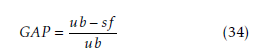
Table 4 examines the results just from the exact For each scenario, this gap is computed as in Equation approach, using CPLEX (without and with an initial

Table 6: Mean Time Delay between generation and consumption of IGRs chosen to be routed, for each solution approach. For those cases where CPLEX is not able to find a feasible solution within the time-limit for any scenarios, the entry is left blank. The results are shown as mean:standard deviation.

Num.		CPLEX w/out	Heuristic	CPLEX w/
Resources	Density	Init Soln		Init Soln
3	1	8.956:0.758	5.070:1.120	8.937:0.738
3	0.67	9.691:1.387	4.968:0.897	9.658:1.389
3	0.33	10.223:0.993	4.651:0.722	10.194:0.960
4	1	9.268:0.954	4.105:0.335	9.278:0.952
4	0.67	9.867:0.734	5.059:0.680	9.856:0.697
4	0.33	10.096:1.153	6.036:1.208	10.128:1.168
5	1	9.004:0.676	3.773:0.327	9.030:0.663
5	0.67	9.762:0.779	5.073:0.433	9.735:0.756
5	0.33	9.588:1.137	5.321:0.700	9.595:1.128
6	1	9.300:0.571	4.021:0.296	9.270:0.582
6	0.67	9.502:0.988	5.257:0.345	9.571:0.953
6	0.33	9.925:1.093	6.361:0.861	9.944:1.050
8	1	9.201:0.700	4.016:0.247	9.186:0.639
8	0.67	9.233:0.558	4.704:0.340	9.426:0.830
8	0.33	10.047:0.665	6.433:0.560	10.099:0.667
10	1	9.010:0.560	3.807:0.321	9.248:0.613
10	0.67	8.504:0.580	4.517:0.316	8.788:0.658
10	0.33	9.460:0.457	6.117:0.519	9.928:0.984
12	1	8.632:0.482	3.846:0.234	9.242:0.494
12	0.67	8.950:0.458	4.684:0.313	9.324:0.497
12	0.33	9.362:0.603	6.194:0.334	11.301:0.979
15	1	7.573:0.398	3.820:0.122	9.599:0.288
15	0.67	8.590:0.698	4.411:0.204	9.197:0.570
15	0.33	9.449:1.149	5.924:0.569	11.035:0.874
20	1	7.633:0.000	3.688:0.148	9.692:0.348
20	0.67	7.586:0.312	4.376:0.068	9.961:0.541
20	0.33	8.684:0.512	5.866:0.269	10.534:1.066
25	1		3.721:0.096	9.629:0.312
25	0.67		4.366:0.211	10.469:0.287
25	0.33	8.471:0.424	5.537:0.139	10.359:1.046

(34), where ub is the upper bound on the solution value and sf is the solution found by CPLEX. We note that when CPLEX finds the optimal solution, ub = sf and the GAP is therefore 0, and when CPLEX is not able to find even a feasible solution, we assigned the trivial solution of sf = 0 (the worst feasible solution for the model), resulting in a GAP value of 1.

What is apparent from Columns 4 and 7 of Table 4 is that CPLEX with an initial solution performs better most of the time as compared to CPLEX without an initial solution. In most cases, there is a significant decrease in the mean gap. However, there are a few cases that are counter-intuitive. Specifically when the number of resources is 6, 8, or 10 and the densities are 0.67, 0.33, or 0.33 respectively. For these three combinations, CPLEX without an initial solution has a smaller mean gap than does CPLEX with an initial solution. This is because there was one scenario in each of these combinations where the heuristic found a solution not close to the optimal, and CPLEX had a difficult time given the heuristic solution as the initial solution, i.e., the heuristic found a local maximum, and CPLEX had a difficult time finding a solution better than this local maximum.

Table 5 shows the average normalized distances between the heuristic solutions and the CPLEX solutions without and with the initial solution. Each normalized distance is computed according to Equation (35),

Table 7: Average runtime (in seconds) for each solution approach to find a solution. For those cases where CPLEX is not able to find a feasible solution within the time-limit, the returned time by CPLEX is still used in this computation. Num. CPLEX w/out Heuristic CPLEX w/ Resources Density Init Soln Init Soln 3 1 218.705 0.002 224.092 3 0.67 48.794 0.000 132.075 3 0.33 10.150 0.000 12.552 4 1 22.205 0.003 30.301 4 0.67 179.300 0.000 190.852 4 0.33 123.936 0.001 155.227 5 1 388.937 0.000 337.506 5 0.67 433.410 0.002 498.094 5 0.33 465.390 0.001 444.524 6 1 469.135 0.002 634.885 6 0.67 595.497 0.002 502.483 6 0.33 109.626 0.000 161.185 8 1 901.857 0.008 901.757 8 0.67 901.863 0.006 865.321 8 0.33 822.245 0.005 761.825 10 1 904.283 0.006 903.338 10 0.67 905.129 0.005 905.198 10 0.33 903.219 0.002 903.443 12 1 904.817 0.011 905.141 12 0.67 905.752 0.003 906.519 12 0.33 905.980 0.003 904.835 15 1 910.124 0.044 910.081 15 0.67 1310.217 0.005 1071.725 15 0.33 1161.690 0.005 1124.190 20 1 2872.113 0.083 2066.906 20 0.67 1283.765 0.009 994.237 20 0.33 958.069 0.005 1153.269 25 1 4612.964 0.128 2845.093 25 0.67 6458.231 0.006 6317.989 25 0.33 1672.833 0.006 1980.635

where {x_j^h,s_j^h} is the solution found by the heuristic, {x_j^c,s_j^c} is the solution to the linearized formulation using CPLEX, and f is the objective function. Since we have a maximization problem, values of Equation (35) larger than 0 indicate that the heuristic is finding a better solution than is CPLEX, while those less than 0 indicate an heuristic solution worse than that found by CPLEX. First off, as expected, all of the values in the last column of Table 5 are negative, because the worst solution ‘CPLEX with initial solution’ can find is the same solution as found by the heuristic since this is the solution provided as input to CPLEX. For less than 12 resources, CPLEX without an initial solution is also able to find a better solution on average than is the heuristic. However, after this point, for almost all cases the heuristic is finding a better solution than is CPLEX without an initial solution. Again, this is to be expected, because as the size of the problem grows, commercial software will have more difficulty in solving the larger problems and the heuristic will begin to find better solutions. But in comparing the heuristic with CPLEX with an initial solution, the average normalized distance between solutions is never that large on average, showing that the heuristic is able to find a good-quality solution as compared with commercial software.

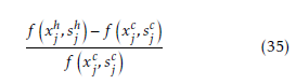Table 6 presents, for those IGRs chosen to be routed, the mean time delay between IGR generation and IGR consumption. Column 3 of Table 6 shows the mean delay for the CPLEX solution when no initial solution is provided, Column 4 shows the mean delay for the heuristic solution, while Column 5 shows the mean delay for the CPLEX solution when an initial solution is provided. As is clear from this table, for those IGRs routed, the heuristic is able to route them much quicker than is CPLEX. This is regardless of the size of the problem. The rationale for this is that the heuristic is choosing IGRs to route in a greedy way, while CPLEX considers the routing of all IGRs simultanously.

Table 7 presents the average runtime for each of the approaches, in seconds. As is clear, the developed heuristic is quite fast in finding solutions for all of the scenario classes. It is also clear that the heuristic takes longer to run on average when the communication network topology is dense as opposed to sparse. Both of the CPLEX approaches take much longer than does the heuristic. Even when the number of resources is as small as 8, these approaches reach (or almost reach) the time limit of 900 seconds. Hence, to get sightly better solutions (according to the objective function) CPLEX needs much more time than does the heuristic. We note that while CPLEX was given a time limit of 900 seconds, there were cases where CPLEX does take longer to complete. This is due to CPLEX not being able to ‘halt’ processing exactly when the time limit is reached.

5. Conclusions and Future Research

In this research, we have examined the problem of routing information amongst a set of resources, when there exists a dynamic communication network topology with limited, time-varying, bandwidth, over a given time horizon. A rigorous mathematical formulation was developed to model the problem, with the objective being to minimize the time delay of the information that can be routed while at the same time maximizing the size of the information routed. This formulation is nonlinear, but a linearized version can be derived through standard techniques of operations research. As the problem is NP-hard, a heuristic has been developed to efficiently find good-quality solutions. Numerous Monte-Carlo simulations were performed on problems with varied resources and communication network topology density. As can be seen in the results, for smaller sized problems commercial software is able to find a better solution on average than is the heuristic. And when the commercial software uses as input the solution found by the heuristic, even better results are obtained. As the size of the problem increases, however, the heuristic begins finding much better solutions compared with the commercial software. And even when the commercial software is provided the heuristic solution as input, the commercial software is not able to improves significantly on this solution. Looking at the metric of the actual timedelay for those IGRs chosen to be routed, it is clear that the heuristic is better able to route those chosen IGRs. When coupled with the time needed for the heuristic to find a good quality solution versus the commercial software, it is clear that the heuristic is outperforming the commercial software.

Future research includes looking at specific network topology structures from realistic military and civil applications, considering the related problem of finding the minimum network temporal connectivity necessary to ensure certain information is able to be routed within time bounds, as well as considering the problem from a decentralized control paradigm, when no resource has knowledge about the network as a whole, but rather must consider only local network knowledge and make independent routing decision. In addition, incorporating the concept of network packet errors will provide added complexity and realism to the problem and scenarios considered.

Conflict of Interest

The authors declare no conflict of interest.

Acknowledgment

This research was Supported by Office of Naval Research Project N00014-15-C-5163.

1.  M. J. Hirsch, A. Sadeghnejad, and H. Ortiz-Pena, “Shortest paths for routing information over temporally dynamic communication networks,” in Proceedings of the IEEE Military Communications Conference, pp. 587–591, 2017.
2.  I. Akyildiz, W. Su, Y. Sankarasubramaniam, and E. Cayirci, “Wireless sensor networks: A survey,” Computer Networks, vol. 38, pp. 393–422, 2002.
3.  J. Al-Karaki, , and A. Kamal, “Efficient virtual-backbone routing in mobile ad hoc networks,” in Elsevier Computer Networks, vol. 52, pp. 327–350, 2008.
4.  E. Huang, W. Hu, J. Crowcroft, and I. Wassell, “Towards commercial mobile ad hoc network applications: a radio dispatch system,” 6th ACM International Symposium on Mobile Ad Hoc Networking and Computing, pp. 355–365, 2005.
5.  “Army 18.1 Small Business Innovation Research (SBIR) Proposal Topic 025: An Adaptively Covert, High Capacity RF Communications / Control Link,” tech. rep., 2018.
6.  “Air Force 18.1 Small Business Innovation Research (SBIR) Proposal Topic 019: Novel Battle Damage Assessment Using Snesor Networks,” tech. rep., 2018.
7.  C. Howard, “UAV command, control, and communication,” Military and Aerospace Electronics, vol. 24, 2013.
8.  B. Vignac, F. Vanderbeck, and B. Jaumard, “Reformulation and decomposition approached for traffic routing in optical networks,” Networks, vol. 67, pp. 277–298, 2016.
9.  J. Brodkin, “Tropical storm Harvey takes out 911 centers, cell towers, and cable networks,” ars Technica, August 28 2017.
10.  L. K. Comfort and T. W. Haase, “Communication, choerence, and collective action: The impage of Hurrican Katrina on the communication infrastructure,” Public Works Management & Policy, vol. 11, no. 1, pp. 1–16, 2006.
11.  U.S. Air Force, “USAF Strategic Master Plan,” tech. rep., 2015.
12.  “Air Force 17.1 Small Business Innovation Research (SBIR) Proposal Topic 047: Resilient Communication for Contested Autonomous Manned/Unmanned Teaming,” tech. rep., 2017.
13.  D. L. Hall and J. Llinas, “An introduction to multisensor data fusion,” in Proceedings of the IEEE, vol. 85-1, pp. 6–23, 1997.
14.  E. Bosse, J. Roy, and S. Wark, eds., Concepts, Models, and Tools for Information Fusion. Artech House, 2007.
15.  F. A. A. U.S. Department of Transportation, “Aviation Maintenance Technician Handbook – Airframe, Volume 2,” tech. rep., 2012.
16.  “Navy 17.A Small Business Technology Transfer (STTR) Proposal Topic T029: Multi-Vehicle Collaboration with Minimal Communication and Minimal Energy,” tech. rep., 2017.
17.  I. Jebadurai, E. Rajsingh, and G. Paulraj, “Enhanced dynamic source routing protocol for detection and prevention of sinkhole attack in mobile ad hoc networks,” International Journal of Network Science, vol. 1, pp. 63–79, 2016.
18.  U. Paul, M. Buddhikot, and S. Das, “Opportunistic traffic scheduling in cellular data networks,” IEEE International Symposium on Dynamic Spectrum Access Networks, pp. 339–349, 2012.
19.  J. Al-Karaki, R. Ul-Mustafa, and A. Kamal, “Data aggregation and routing in wireless sensor networks: Optimal and heuristic algorithms,” in Elsevier Computer Networks, vol. 53, pp. 945–960, 2009.
20.  M. J. Hirsch, H. Ortiz-Pena, R. Nagi, A. Stotz, and M. Sudit, “On the optimization of information workflow,” in Dynamics of Information Systems: Mathematical Foundations (A. Sorokin, R. Murphey, M. Thai, and P. Pardalos, eds.), vol. 20, pp. 43–65, Springer, 2012.
21.  M. J. Hirsch and H. Ortiz-Pena, “Information supply chain optimization with bandwidth limitations,” International Transactions in Operational Research, vol. 24, no. 5, pp. 993–1022, 2017.
22.  E. Grotli and T. Johansen, “Path and data transmission planning for cooperating uavs in delay tolerant network,” in Globecom Workshop, pp. 1568–1573, IEEE, 2012.
23.  S. Basagni, C. Petrioli, R. Petroccia, and M. Stojanovic, “Optimizing network performance through packet fragmentation in multi-hop underwater communications,” in OCEANS, pp. 1–7, IEEE, 2010.
24.  P. Kansal and A. Bose, “Bandwidth and latency requirements for smart transmission grid applications,” IEEE Transactions on Smart Grid, vol. 3, pp. 1344–1352, 2012.
25.  M. Greenberg, Advanced Engineering Mathematics. Pearson, 2nd ed., 1998.
26.  L. Wolsey, Integer Programming. Wiley, 1998.
27.  I. CPLEX, “http://www-01.ibm.com/software/commerce /optimization/cplex-optimizer/,” Accessed January 2017.
28.  LINDO, “http://www.lindo.com/,” Accessed July 2016.
29.  J. Lenstra and A. R. Kan, “Complexity of vehicle and scheduling problems,” Networks, vol. 11, pp. 221–227, 1981.
30.  M. Solomon and J. Desrosiers, “Time window constrained routing and scheduling problem,” Transportation Science, vol. 22, pp. 1–13, 1988.
31.  M. Dror and P. Trudeau, “Split delivery routing,” Naval Research Logistics, vol. 37, pp. 383–402, 1990.
32.  G. Ausiello, M. Protasi, A. Marchetti-Spaccamela, G. Gambosi, P. Crescenzi, and V. Kann, Complexity and Approximation: Combinatorial Optimization Problems and Their Approximability Properties. Springer-Verlag New York, Inc., 1st ed., 1999.
33.  M. R. Garey and D. S. Johnson, Computers and Intractability: A Guide to the Theory of NP-Completeness. New York, NY, USA: W. H. Freeman & Co., 1979.
34.  Matlab, http://www.mathworks.com/products/matlab/, Accessed January 2017.
35.  B. Szymanski, X. Lin, A. Asztalos, and S. Sreenivasan, “Failure dynamics of the global risk network,” Scientific Reports, vol. 5, pp. 1–14, 2015.
36.  R. Liu, M. Li, and C. Jia, “Cascading failures in coupled networks: The critical role of node-coupling strength across networks,” Scientific Reports, vol. 6, pp. 1–6, 2016.
37.  K. Kim, J. Jin, and S. Jin, “Classification between failed nodes and left nodes in mobile asset tracking systems,” Sensors, vol. 16, pp. 1–18, 2016.

(Click Here)

(Click Here)