1. Introduction

Nowadays, the biological processes become one of the important industrial processes thanks to their advantages, such as the treatment of organic substrates, protein production and the production of ethanol gas etc. However, their modeling and control form a real challenge problem for both control engineers and theorists, where this kind of systems are characterized by strong variations of system parameters and unknown kinetics owing to the time-varying characteristics and multiple interactions generated by the living microorganisms [1, 2]. Therefore, we obtain a highly nonlinear system. The motivation of this work is to linearize the model and benefit from linear theory control and to try to develop a nonlinear control, which is very difficult in this case. Also to use the Takagi-Sugeno (T-S) model, furthermore, the proposed controllers can be applied to the real process. It only needs to identify a T-S model from experimental data. T-S approach has been recognized as an effective tool for handling the previous difficulty.

There are different techniques for controlling the bioprocess using Takagi-Sugeno models, such as optimal fuzzy linear quadratic regulators for discrete-time [3], a fuzzy integral controller to force the switching of a bioprocess between two different metabolic states is treated in [4], an internal model control design strategy is developed for a particular Continuous Stirred-Tank Reactor (CSTR)[5]. A PID and fuzzy controller are proposed in [6] to stabilize the CSTR around the equilibrium point, where the authors consider only one input, which is not the case in practice. Also, the case of uncertain Takagi-Sugeno system is treated in [7], where an observer with unmeasurable premise variables and unknown input is considered for a wastewater treatment plant. In addition, the predictive control based on fuzzy observer is studied for a sludge depollution bioprocess in [8, 9], in this framework one can cite [10, 11, 12]. Furthermore, the modeling and the control of bioprocess based on neural network approach is treated in [13, 14]. In the same spirit, a nonlinear model autoregressive with exogenous input model predictive control is developed in [15] to control the fermentation process. Also, an integral backstepping control law is developed in [16] for controlling the dissolved oxygen level for bacteria fermentation.

The problem treated in this paper is how to model and control the biomass growth process, ensuring the trajectory tracking while taking into account the following constraints:

• The mathematical model is nonlinear and not affine in control.
• The variables control present the physical constraints, which make the computation of the control gains difficult.
• The full system states are not measurable. The present paper has two goals, the first is to build a fuzzy model of biological process based on TakagiSugeno tool, especially the nonlinearity sector methods. The second is to ensure the tracking trajectory of the desired outputs using two approaches: the Parallel Distributed Compensation (PDC) [17] and the Linear Quadratic Integral (LQI) control. Where the strong physical constraints on the inputs [18] are taking into account. In addition, the proposed controllers are compared. The stability conditions are formed in the Linear Matrix Inequalities (LMIs) terms.

This paper is organized as follows: Section 2 presents the description of the Takagi-Sugeno modeling. Section 3 describes the parallel distributed compensation control. Then, one can address the fuzzy output tracking control problem in section 4 and we show that it can be solved by using two methods: the PDC technique and the optimal linear quadratic control. Section 5 describes the controller design based on fuzzy observer with unmeasurable premise variables. Section 6 introduces the proposed biological process. Finally, the simulation and the discussion of the obtained results are given to compare the proposed controllers.

2. Takagi-Sugeno Fuzzy Model

In order to extend the existing approaches of control and observation for linear to nonlinear system, Takagi and Sugeno have proposed a fuzzy dynamic model to represent this kind of system. The T-S fuzzy model is a set of linear models connecting via membership functions. To build the T-S fuzzy model, three methods exist in the literature [17]: The black box identification, the linearization method and the nonlinearity sector methods. The third method gives an exact T-S representation of nonlinear system without information loss.

Consider the following nonlinear system:

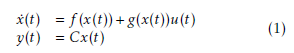where x ∈ _Rⁿ is the state, u ∈ _R^m is the input vector, y ∈ _R^q represents the output measurement vectors and C ∈ _R^q∗n is the output matrix. In addition, f (.) and g(.) represent the nonlinear functions. The T-S fuzzy model uses a set of fuzzy if-then rules, which represent local linear input-output relations of a nonlinear system. The i^th rule of the T-S model given as follows:

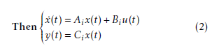Where F_pⁱ are the membership functions of fuzzy sets, i ∈ {1,2,…r }, r is the number of rules, A_i ∈ _R^n∗n, B_i ∈ _R^n∗m, C_i ∈ _R^q∗n and z₁(t),…,z_p(t) are the premise variables which can be dependent of the input, the output or the state. The global T-S fuzzy model is given in the following form:

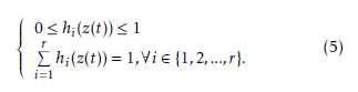
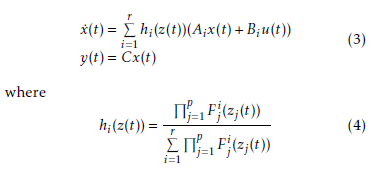The activation functions h_i(z(t)) indicates the activation degree of the i^th associated local model, this functions verifies all time the convex sum propriety:

3. PDC control approach

3.1. Fuzzy regulator design via PDC

To stabilize the system presented by their T-S fuzzy model, the PDC controller is usually used to design a fuzzy controller. The main idea is to design a local controller for each sub-model based on local control rule, which shares with the fuzzy model the same fuzzy sets. The overall fuzzy controller is represented by:

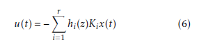Where the K_i represent the local feedback gains. by using (6) in (3) the system in closed-loop becomes:

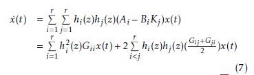with G_ij = A_i − B_iK_j, the stability conditions of (7) are given by the following theorem [17].

Theorem 1 The continuous fuzzy system (7) is asymptotically stable, if there exist a common positive matrix P ∈ R^n×n and a common positive semi definite matrix

Q ∈ R^n×n and for a number of active rules s, where 1 < s ≤ r such that:

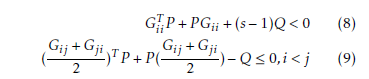In order to transform the preview conditions into LMIs form, one can consider the following variables: X = P ⁻¹

, K_i = M_iX⁻¹ , Q = P YP , where X > 0, Y ≥ 0 and

M_i(i = 1,…,r), then the stabilization conditions become:

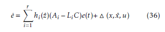
The trajectory tracking control of nonlinear systems is the subject this section. In the tracking loop, we consider the integral of the tracking error e_I = ^R (y_r − y)dt =

R

(y_r − Cx)dt [19], with y_r is the desired output. If we consider the following augmented state:

” # x

Xa = eI

Then, the following augmented system is obtained:

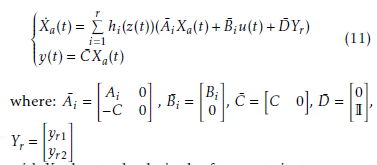Yr = yy_rr₂1 with Y_r, denote the desired reference trajectory.

4.1. PDC control

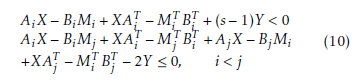
To achieve the output tracking, the state feedback PDC control based on the previous LMIs can be used. The fuzzy controller u(t) has the same form of (6), where x is replaced by the augmented state X_a:

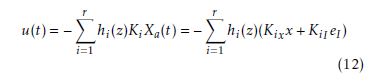The feedback gains of the controller K_i = K_ix K_iI are obtained by solving the LMIs (10).

4.2. LQI control

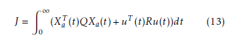
To design the LQI control, the following quadratic cost criterion must be minimized by the control law u(t):

0 for this reason, the following candidate quadratic Lyapunov function is considered:

V (Xa) = XaT P Xa The augmented system (7) is stable if :	(14)
XaT QXa +uT Ru +V˙ (Xa) < 0	(15)

            (A¯_i +B¯_iK_i)^T P_i +P_i(A¯_i +B¯_iK_i)+Q +K_i^T RK_i < 0              (16)

(A¯_iX_i +B¯_iY_i)^T +(A¯_iX_i +B¯_iY_i)+X_iQX_i +Y_i^T RY_i < 0 (17)

(A¯iXi +B¯iYi)T +(A¯iXi +B¯iYi)+YiT RYi − Xi(−Q)Xi < 0

(18)

by using the Schur complement procedure, the following stability conditions are obtained:

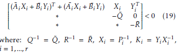where: Q−1 = Q˜, R−1 = R˜, Xi = Pi−1, Ki = YiXi−1, i = 1,…,r

This LMIs will be calculated for each sub-model, here is about the conventional linear quadratic integral control using the fuzzy model. The control law is not based on fuzzy rules.

The control law will be respect the physical constraints on the control input, where this problem is studied in many practical cases [20, 21, 22, 23]. To ensure the stabilization under constraints on the inputs, the conditions given in the following theorem [17] must be verified.

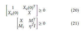
Theorem 2 For a known initial condition X_a(0), the constraint ku(t)k₂ ≤ η is enforced at all times t ≥ 0 if the LMIs:

4.3. Observer design

In bioprocess control problems, the state variables are not usually available. By introducing the observer, one can reconstruct partially or all the state variables. This section presents the fuzzy observer design with unmeasurable premise variables z(t) (h_i(z) , h_i(zˆ)). Based on the structure of the fuzzy model (3), the fuzzy observer is given as follows:

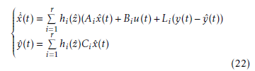where xˆ denotes the estimated state and L_i the gains of the observer.

In order to compute this gains the following theorem [24] gives the necessary conditions for ensuring the convergence of the state estimation error to zero.

Theorem 3 If there exist symmetric and definite positive matrices P ∈ Rn×n, Q ∈ Rn×n, matrices Yi ∈ Rn×q and a scalar α > 0 such that:

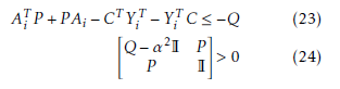then, the estimation error between the T-S fuzzy model (3) and the fuzzy observer (22) is converges asymptotically to zero. where: L_i = P ⁻¹Y_i.

Proof 1 See Appendix.

5. Process description

The proposed biological process in this paper is a biomass growth process, which consists to grow the population of microorganisms (biomass) by the consumption of a substrate (glucose), according to the following reaction scheme:

The dynamic model of this process is established from the mass-balance [25], which describes the evolution of substrate and biomass concentrations in a continuous bioreactor. This model can be represented by a high nonlinear system as follows:

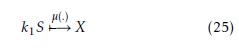
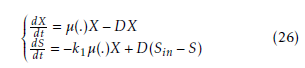The state variables are the biomass X and substrate S concentrations, k₁ denotes the pseudo stoichiometric coefficient and µ(.) represent the specific growth rate, the ”Monod law” characterizes µ(.) is:

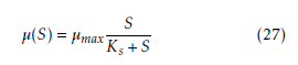where µ_max is the maximum specific growth rate; K_s is the Monod or saturation constant. The input variables are the dilution rate D(t) and the influent substrate concentration S_in. The parameters of the proposed model are given in the Table 1.

Parameters	Value	Unit
µmax	0.38	h−1
Ks	5	g/l
k1	1/0.07
Smax	140	g/l

Table 1: Simulation parameters

5.1        Takagi-Sugeno model design

The model (26) must be transformed into affine in control model like in (1), where the bioprocess models are known belong to the class of affine nonlinear models, this can be easily shown by assuming that:

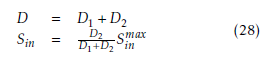where D₁(t) and D₂(t) are respectively the water and the substrate dilution rate, then one can replace D(t) and S_in(t) in (26) by their expressions (28), the following affine model is obtained:

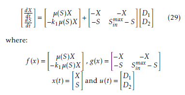To build the T-S model, the following nonlinearities are considered:

z1(x) = µ(S)	(30)
z2(x) = X	(31)
z3(x) = S	(32)

A(z) = −kz11z1 00 and B(z) = −−zz23 −z3 −+zS2inmax where the number of nonlinarities n = 3, the global model can be represented by r = 2ⁿ = 8 sub-models. The local membership functions are defined by:

            F11(z1) = z1maxz1−−z1minz1min , F12(z1) = z1maxz1max−−z1minz1

z2−z2min

                 F21(z2) = z2max−z2min , F22(z2) = z2maxz2max−−z2minz2

z₃−z³min , F₃2(z3) = _z3maxz³max₋−_z3minz₃ F₃1(z3) = _z3max_−z3min

Finally, the activation functions are:

h1(z) = F11(z1)F21(z2)F31(z3), h3(z) = F11(z1)F22(z2)F31(z3), h5(z) = F12(z1)F21(z2)F31(z3), h7(z) = F12(z1)F22(z2)F31(z3),

h2(z) = F11(z1)F21(z2)F32(z3) h4(z) = F11(z1)F22(z2)F32(z3) h6(z) = F11(z1)F21(z2)F32(z3) h8(z) = F12(z1)F22(z2)F32(z3)

For the simulation, the parameters given in Table 1 are considered and leads to the following min and max of

premise variables:
0.018	≤ µ(S) ≤ 0.35
3.8	≤ X ≤ 20
0.6	≤ S ≤ 140

the computed matrix A_i and B_i of each sub-model are given as follows:

”                       # 0.3507     0 A1 = A3 = A5 = A7 = −5.0106  0 ”                       # 0.0179     0 A2 = A4 = A6 = A8 = −0.2551  0
”                      #                     “ −20      −20                           −3.8 B1 = B2 = −140             0        ,B3 = B4 = −140	−3.8# 0
”                        #                     “ −20    −20         −3.8 B5 = B6 = −0.6                139.4 ,B7 = B8 = −0.60	−3.8 # 139.4

6. Simulation and results

In the first case, all the states variables (substrate and biomass concentrations) are supposed measurable (i.e.

The desired trajectory (X_r and S_r), which represent respectively of biomass and substrate concentrations are computed by using the following reference model:

X˙˙_r == −−00..6597SX_rr+0+0.65.97refref_SX (33) S_r where ref_X and ref_S are the setpoints.

6.1. Tracking control based on state feedback

6.1.1. PDC control

The studied bioprocess presents the physical constraints on the control as shown in the Table 2

Variables	Constraints
Dilution rate h−1	0.01 6 D 6 0.38
Influent substrate g/l	60 6 Sin 6 140

Table 2: The control constraints

For a number of active sub-model s = 5 and η =

1.55, the LMIs (10), (20) and (21) are solved by using the solver SeDuMi in MATLAB toolbox YALMIP, gives the following gains:

” 0.0384 K1 = −0.2821	−0.0044 0.0064	−0.0007 0.0564	0.0083 # −0.0088
” 0.0052 K2 = −0.2472	−0.0044 0.0064	−0.0007 0.0563	0.0083 # −0.0088
“0.03470 K3 = −0.2963	−0.0044 0.0064	0.0002 0.05930	0.0083 # −0.0088
” 0.0011 K4 = −0.2605	−0.0044 0.0064	0.0002 0.05910	0.0083 # −0.0088
“ −0.2149 K5 = −0.0287	−0.0010 0.0044	0.0572 −0.0014	0.0074 # −0.0083
“−0.2480 K6 =         0.0060	−0.0010 0.0044	0.0571 −0.0015	0.0074 # −0.0083
” −0.22450 K7 =             −0.0371	−0.0009 0.0044	0.0592 0.0003	0.0074 # −0.0083
” −0.25660 K8 =             −0.0028	−0.0009 0.0044	0.0590 0.0003	0.0074 # −0.0083
 0.0059  −0.0000   P =−0.0011     0.0000	−0.0000 0.0008 0.0000 −0.0002	−0.0011 0.0000 0.0008 −0.0000	0.0000   −0.0002  −0.0000 0.0008 
 7.5254    0 Q = 2..00029997    −0.0011	0.0002 35.5015 0.0002 0.0002	2.9997 0.0002 23.9724 0.0013	−0.0011  0.0002   0.0013  26.1931

The initial conditions are x₀ = (6.6 5.50)^T and the obtained results are shown in Figures 1 and 2, the trajectory tracking is achieved, where the biomass and the substrate concentrations follow the desired outputs. In addition, the constraints on the inputs control D(t) and S_in(t) are respected.

Figure 1: Evolution of the system outputs

Figure 2: Control inputs D(t) and S_in(t)

6.1.2. LQI control

Solving the LMIs established in (19), (20) and (21) the obtained weighting matrices are:

                   ” 0.0202       −0.0081     0.0044       0.0101 #

            ^{K1 =} −0.0736         0.0128      0.0098     −0.0056

” 0.0010 K2 = −0.0368	−0.0095 0.0052	0.0010 0.0195	0.0105 # −0.0030
” 0.0317 K3 = −0.2002	−0.0095 0.0039	0.0008 0.0165	0.0106 # −0.0004
” 0.0016 K4 = −0.1086	−0.0096 0.0023	0.0002 0.0271	0.0106 # −0.0005
“ −0.0247 K5 =              −0.031	−0.0003 0.0095	0.0211 −0.0006	0.004 # −0.009
“ −0.0345 K6 = −0.0024	−0.0050 0.0096	0.0200 0.0009	0.0033 # −0.0105
“ −0.1471 K7 = −0.0369	−0.0047 0.0095	0.0211 0.0003	0.0035 # −0.0105
“ −0.1064 K8 = −0.0023	−0.0026 0.0096	0.0274 0.0003	0.0009 # −0.0107

The Figures 3 and 4 show the simulation results using LQI control, where the controlled outputs variables achieve the desired outputs, also the constraints on control are respected.

Figure 3: Evolution of the system outputs

Figure 4: Control inputs D(t) and S_in(t)

The results obtained are comparable or even better than those obtained using the PDC controller.

6.2. Tracking control based on reconstructed state feedback

In the practical case, only the substrate concentration is measured and the biomass is estimated, then the out-

h               i put matrix in (1) becomes C = 0      1 . For the initial conditions of system x₀ = (4 8)^T , the initial conditions of observer xˆ₀ = (5       7)^T and for a scalar α = 0.5, the following observer gains are obtained:

” 5.2458 #

L1 = L3 = L5 = L7 = −1.3202

” 0.3483 # L2 = L4 = L6 = L8 = −0.6440

5.655  Q = 0.000  −0.00	0.000 4.4141 0.000	−0.000  0.000  6.2045
0.5985  P = 0.0843  0.0000	0.0843 0.6103 0.0000	0.0000  0.0000 0.6103

6.2.1. PDC control

The resolution of the same LMIs in last case gives the following gains.

” 0.0231 K1 = −0.1294	−0.0043 0.0058	0.0067 # −0.0037
“ −0.0057 K2 = −0.1082	−0.0044 0.0058	0.0066 # −0.0033
” 0.0304 K3 = −0.1425	−0.0044 0.0058	0.0064 # −0.0027
“ −0.0038 K4 = −0.1187	−0.0045 0.0058	0.0065 # −0.0031
“ −0.0814 K5 = −0.0336	−0.0015 0.0044	0.0094 # −0.0065
“ −0.1090 K6 = −0.0016	−0.0015 0.0044	0.0092 # −0.0064
“ −0.0857 K7 = −0.0359	−0.0018 0.0048	0.0096 # −0.0065
“ −0.1151 K8 = −0.0036	−0.0015 0.0046	0.0094 # −0.0064
 0.0114  P =−0.0001  −0.0003	−0.0001 0.0010 −0.0002	−0.0003  −0.0002 0.0008 
 0.0114  Q =−0.0001  −0.0003	−0.0001 0.0010 −0.0002	−0.0003  −0.0002 0.0008 

The Figure 5 shows a comparison between the controlled variable S, his estimated Sˆ and the desired output S_r. The obtained result show that S follows correctly S_r and the observer estimates the states of system (Sˆ = S) after 4.33 hours. The Figure 6 presents the control inputs D(t) and S_in(t), which respect the constraints.

Figure 5: Evolution of the system outputs

Figure 6: Control inputs D(t) and S_in(t)

6.2.2. LQI control

In this part, we illustrate the obtained results using LQI control. Solving the LMIs (20), (21), (19) we obtain the following controller gains and weighting matrices:

 0.1138  Q = 0.0012  −0.0009		0.0012 0.1360 −0.0196		−0.0009  −0.0196.10−3 0.1072 
” 0.0000 K1 = −0.0566		−0.0043 0.0087		0.0066 # −0.0035
” 0.0015 K2 = −0.0124		−0.0076 0.0015		0.0067 # −0.0001
” 0.0182 K3 = −0.1308		−0.0072 0.0032		0.0069 # −0.0003
	” 0.0017 K4 = −0.0222		−0.00760      0.0067# 0.0003             0.0002
	“ −0.0130 K5 = −0.0231		0.0005 0.0071		0.0032 # −0.00560
	“ −0.0105 K6 = −0.0016		−0.0017 0.0076		0.0009 # −0.0067
	“ −0.0624 K7 = −0.0327		−0.0034 0.0073		0.0027 # −0.0062
	“ −0.0204 K8 = −0.0018		−0.0009 0.0076		0.0004 # −0.0067

The Figures 7 and 8 present the same variables in the Figures 5 and 6 using the LQI control. where the obtained results indicate clearly that the desired performances can be achieved more better than the results obtained by PDC control, the Figure 9 shows the state estimation error of the state variables ( biomass and substrate concentrations), where this error tends to zero after 4.33 hours.

Figure 7: Evolution of the system outputs

Figure 8: Control inputs D(t) and S_in(t)

Figure 9: The sate estimation error

6.3.  Comparison of both controllers

The outputs behaviors in the Figures 1, 3, 5, 7, show that the PDC controller presents some overshoot compared with LQI controller, where the PDC control requires the stabilization of all the different sub-models cross terms (h_i(z) , h_j(z)) too, which increases the LMIs need to be solved. Moreover, in terms of speed, the comparison shows clearly that the LQI controller is fast than PDC one. In general, the comparison shows that the LQI controller presents the best performance.

6.4. Comparison with other methods

Another method of bioprocess control based on neural network model has been developed in [13], where the process is controlled via a neural predictive controller in that case the controller doesn’t refer to a mathematical model for the process but consider the black box identification. In our case we are based on the mathematical model for the synthesis of the controller, the obtained results are satisfactory regarding the result obtained in [13]. Another work in the same spirit developed by A. Nikfetrat [14], where the study considers a predictive controller applied to a biological feed-batch process without taking into account the constraints on the input variables and shows an important error in tracking reference trajectories, where the present work gave better results.

7. Conclusion

In this paper, the modeling and the control of the biomass growth process are treated. The objective is to control and compare two controllers. The nonlinear model of this process obtained from the mass-balance is transformed to Takagi-Sugeno fuzzy model, which represents exactly the original nonlinear model. Then, a T-S observer is designed to reconstruct the unmeasurable state when the premise variables are not measurable. To ensure the trajectory tracking two controllers are tested. The PDC and the linear quadratic control. The obtained results show that the two controllers are both effective. Finds that the second controller is more stable. In addition, the inputs respect the physical constraints of the process.

In this study, we only focus on the bioprocess control in faulty free case, that is why one interesting future work is to build a fault-tolerant control for this process.

Appendix

The proof of the Theorem 3 is presented here, we consider the following state estimation error:

                                      e(t) = x(t) − xˆ(t)                                (34)

their dynamic becomes:

e˙(t) =x˙(t) − xˆ˙(t)

we take:

the error dynamic then becomes:

if we assume that the term M (x,x,u ) satisfies the condition of Lipschitz as follows:

                               ^k M (x,x,uˆ )^{k ≤} α ^kx ⁻ xˆ ^k                       (37)

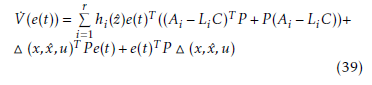
to ensure the convergence of (36) , one can consider the following candidate quadratic Lyapunov function:

                                   V (e(t)) = e(t)^T P e(t)                             (38)

leads to:

Lemma 1 For two real matrices X and Y of appropriate dimensions, the following inequality is verified:

X^T Y +XY ^T < X^T Ω⁻¹X +YΩY ^T ,Ω > 0

Applying the previews lemma to the term: M (x,x,uˆ )^T P e(t) + e(t)^T P M (x,x,uˆ ) , the derivative of (39) is expressed as:

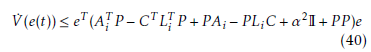If there exists a symmetric and positive definite matrix Q = Q^T such that:

leads to:

Finally, we apply the Schur complement to (42) we obtain:

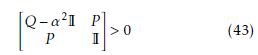Then the proof is completed.

1.  V. Vastemans, M. Rooman, P. Bogaerts, “A robust method for the joint estimation of yield coeffcients and kinetic parameters in bioprocess models”, Biotechnology Progress 25 (3), 2009, 606–618. doi:10.1002/btpr.89.
2.  A. Karama, O. Bernard, J.-L. Gouz´e,“ Constrained Hybrid Neural Modelling of Biotechnological Processes”, International Journal of Chemical Re- 70 actor Engineering 8 (1), 2010, 1–15. doi:https://doi.org/10.2202/ 1542-6580.2117.
3.  V. Grisales, A. Gauthier, G. Roux, “Fuzzy Optimal Control Design for Dis- crete Affine Takagi-Sugeno Fuzzy Models: Application to a Biotechnologi- cal Process”, 2006 IEEE International Conference on Fuzzy Systems, 2006, 2369–2376, doi:10.1109/FUZZY.2006.1682030.
4.  E. Herrera, B. Castillo, J. Ramrez, E. C. Ferreira, “Takagisugeno multiple- model controller for a continuous baking yeast fermentation process”, ICINCO 2007 – 4th International Conference on Informatics in Control, Automation and Robotics, Proceedings ICSO, 2007, 436–439. doi:10.5220/0001622704360439.
5.  Min-Sen Chiu, Shan Cui, Qing-Guo Wang. “ Internal Model Control Design for Transition Control”, AIChE journal, vol 46, 2000
6.  E. J. Herrera-Liopez, B. Castillo-Toledo, R. Femat, “Fuzzy servo controller 65 for CSTB with substrate inhibition kinetics”, Journal of Process Control 22 (6) (2012) 959–967. doi:10.1016/j.jprocont.2012.05.003.
7.  A. M. Nagy Kiss, B. Marx, G. Mourot, G. Schutz, J. Ragot, “Observers de- sign for uncertain Takagi-Sugeno systems with unmeasurable premise vari- ables and unknown inputs. Application to a wastewater treatment plant”, 30 Journal of Process Control 21 (7), 2011, 1105–1114. doi:10.1016/j. jprocont. 2011.05.001.
8.  M. Bouharkat, M. Ramdani,“ Fuzzy observer based predictive control of an activated sludge depollution bioprocess”, 2013 International Conference on Control, Decision and Information Technologies, CoDIT, 2013, 236–241. doi:10.1109/CoDIT.2013.6689550.
9.  E. Herrera, B. Castilloa, J. Ramrezb, E. C. Ferreirac, “Exact fuzzy observer for a baker’s yeast fermentation process”, IFAC Proceedings Volumes (IFAC- PapersOnline) 10 (1), 2007, 313–318. doi:10.1109/FUZZY.2007.4295502.
10.  S. Aouaouda, M. Chadli, M. T. Khadir, T. Bouarar, “Robust fault tolerant tracking controller design for unknown inputs T-S models with unmeasurable premise variables”, Journal of Process Control 22 (5), 2012, 861–872. doi:10.1016/j.jprocont.2012.02.016.
11.  S. Bououden, M. Chadli, H. R. Karimi, “Control of uncertain highly non- linear biological process based on Takagi- Sugeno fuzzy models”, Signal Processing 108 (2015) 195–205. doi:10.1016/j.sigpro.2014.09.011.
12.  S. Carlos-Hernandez, E. N. Sanchez, J. F. B´eteau, “Fuzzy observers for anaerobic WWTP: Development and implementation”, Control Engineering Practice 17 (6), 2009, 690–702. doi:10.1016/j.conengprac.2008.11. 008.
13.  A. Karama, “Contribution `a la mod´elisation et la commande par r´eseaux de neurones des bioproc´ed`es”, thesis, University Cadi Ayyad, Faculty of Science Semlalia Marrakech, 2004.
14.  A. Nikfetrat, A.R. Vali, V. Babaeipour. “Neural Network Modeling and Nonlinear Predictive Control of a Biotechnological Fed-batch Process”, IEEE International Conference on Control and Automation Christchurch, New Zealand, December 9–11, 2009.
15.  Mohd N, Aziz N. “Performance and Robustness Evaluation of Nonlinear Autoregressive with Exogenous Input Model Predictive Control in Controlling Industrial Fermentation Process”, Journal of Cleaner Production, 2016.
16.  O. Gehan, E. Pigeon, M. Pouliquen, L. Fall, R. Mosrati, “Nonlinear control of dissolved oxygen level for Pseudomonas putida bacterium fermentation”, 15 2016 IEEE Conference on Control Applications, CCA 2016 (2016) 1215– 1220 doi:10.1109/CCA.2016.7587972.
17.  K. Tanaka, H. O. Wang, “Fuzzy Control Systems Design and Analysis”, John Wiley and Sons, Inc., New York, USA, 2001. doi:10.1002/0471224596.
18.  Saifia, D., Chadli, M., Labiod, S., and Guerra, T. M., “ Robust H1 Static Output Feedback Stabilization of T-S Fuzzy Systems Subject to Actuator Saturation”, Int. J. Control Autom. Syst. 10(3), 613–622, 2012
19.  Hassan.K.Khali. “Nonlinear Systems”, second edition, Prentice Hall. United States of America, 1996.
20.  Guechi, El-Hadi, Lauber, Jimmy, Dambrine, Michel, et al., “PDC control design for non-holonomic wheeled mobile robots with delayed outputs”, J. Intell. Robot. Syst. 60(3-4), 395–414, 2010
21.  Xu, Bin, Wang, Shixing, Gao, Daoxiang, et al., “Command filter based robust nonlinear control of hypersonic aircraft with magnitude constraints on states and actuators”, J. Intell. Robot. Syst. 73(1-4), 233–247, 2014
22.  Zhu, Senqiang et Wang, Danwei., “ Adversarial ground target tracking using UAVs with input constraints”, J. Intell. Robot. Syst. 65(1-4), 521-532, 2012
23.  M. Abyad, A. Karama, A. Khalloq, “Fuzzy Takagi-Sugeno Based Modelling and Control For an Alcoholic Fermentation Process”, 3rd International Conference on Electrical and Information Technologies ICEIT, Rabat, Morocco, 2017.
24.  P. Bergsten, R. Palm, D. Driankov, “Fuzzy observers”, 10th IEEE International Conference on Fuzzy Systems. (Cat. No.01CH37297) 2, 2001, doi:10.1109/FUZZ.2001.1009051.
25.  Bastin G. and Dochain D. “On-line estimation and adaptive control of bioreactors”. Elsevier, Amsterdam, 1990.

(Click Here)

(Click Here)