1. Introduction

In recent years, the Internet of things has become a hot research topic in industry and academia. In the developing fifth generation wireless mobile communications, the IIoT is an extremely important application case. The IIoT is particularly important in the application of the fifth generation of wireless communications. In the IIoT wireless communications, there are two different types of radio signals: narrow band (NB) and wide band (WB). In the industrial environment, there are a great quantity of mobile equipments work at WB to transmit surveillance video. Basically, there are an enormous amount of sensors work at NB to obtain all kinds of temperature, humidity or pressure information These signals also have different central frequencies. This paper mainly investigates the wireless channel of industrial environment and it is an extension of work originally presented in 2018 20th International Conference on Advanced Communication Technology [1].

The IIoT generally includes three different layers: application layer, perception layer and network layer. The first layer is to be used intelligent sensing technology, such as various sensors, to collect industrial data anytime and anywhere; the second layer is to be used communication technology, such as the Zig-bee, the Narrow Band Internet of Things (NB-IoT), and so on, to build a communication network. The third layers is to be used data processing and analysis technology, such as cloud computing, and so on, to make deep mining and utilization of these data, and then to realize the management and optimization of the industrial process [2]. At the IIoT network layer, huge amounts of sensors connect to the access point by wireless communication technologies. Wireless communication links will be obstructed and shadowed by industrial equipment or metallic materials in the industrial propagation environments. The propagation of electro-magnetic waves will generate strong reflection due to the role of these obstructions. However, in the industrial propagation case, wireless communication technology has not been completely researched. There are many differences between IIoT and cell communication systems. It is important to get a thorough knowledge of the IIoT wireless channel characteristics.

At present, researches on the influence of modern industrial environment on electromagnetic wave propagation are relatively limited. Reference [3] extracted wireless channel parameters of path loss and time delay power based on the measured data of five factories. Reference [4] studied the characteristics of the typical industrial environment by channel measurement based on manufacturing plant. The related parameters obtained from the average time delay and RMS delay obtained from the 2.4GHz center frequency were found to be dependent on the LOS condition and related to the distribution of metal hindrance. Reference [5] measured four typical factory environments (corridors, offices, laboratories and large industrial manufacturing halls) at 1.9GHz center frequency, and analyzed shadow fading, K factor and delay spread which according with log-normal distribution. Reference [6] considered the large-scale characteristics based on measurement data in several factory buildings. Reference [7] researched NB propagation at 900 MHz, 2400 MHz and 5200 MHz. Reference [8] studied the effects of two important industrial environments on electromagnetic wave propagation, including channel path loss and multipath component (MPCs). One is high absorption environment, the other is high reflection environment. In the same year, reference [9] proposed a broad-band channel model for industrial wireless networks. This model takes into account the influence of noise in the harsh factory environment and uses the first order two state Markov process to describe the characteristics of the typical burst pulse noise in the industrial environment. Authors in reference [10] modelled the industrial wireless channels using Saleh-Valenzuela models. In 2017, reference [11] conducted seven scene measurements at three locations, studied the LOS and OLOS scenarios with a frequency of 5.8GHz, and analyzed the wireless channels.

The main contribution of this paper is to employ a vector signal generator and spectrum analyzer as a channel sounding system to probe realistic automobile factory environments. Three frequency bands, 1.1GHz, 2.55GHz, and 5.8GHz are considered in this paper. The frequency bands of 1.1GHz and 2.55GHz are corresponding to narrow band (NB) (0.8MHz) and 5.8GHz is corresponding to wide band (WB) (8MHz). In the NB case, we consider a special condition that the sensor/actuator (receiver antenna of the channel sounder in our channel measurements) is placed inside the metallic body of a machine, an industrial computer box with the thickness of 2 mm in the measurement. The channel parameters of time dispersion including RMS delay spread, number of MPCs, power difference and the K factor in different scenarios are extracted from the measurement data.

The paper is organized as follows. In Section 2, the system model and measurement system are described. Then raw data are analyzed to show the results of measurement and give the reasonable explanation in Section 3 . In Section 4 the conclusion is given.

2. System model and measurements description

As shown in Figure 1, a vector signal generator (Rhodes &Schwartz SMBV100A) and a spectrum analyzer (Agilent N9010B) are employed as a channel sounder. Two local rubidium clocks are employed to ensure efficiency and accuracy synchro- nization between the Tx and Rx. In Table 1 channel measurement parameters are listed.

As shown in Figure 3, two different propagation types of LOS (100 measurement spots) and OLOS (100 measurement spots) are considered in this measurement. In OLOS propagation case, the wireless links are semi-blocked (shadowed) by metal machines and buildings. And as mentioned in the previous part, a special case is considered that the sensor/actuator (receiver antenna of the channel sounder in our channel measurements) is placed inside the metallic body of a machine, as shown in Figure 2. The dimension of the measurement factory is 120 m×59 m×8 m, the Tx antenna height is 5 m and the Rx antenna height is 1.4m.

Table 1: Measurement Parameters.

Bandwidth Type	Frequency	Bandwidth	Power		Antenna Gain
NB	1.1GHz	0.8 MHz	33dBm	0dBi
NB	2.55GHz	0.8MHz	33dBm	0dBi
WB	5.8 GHz	8MHz	33dBm	16dBi

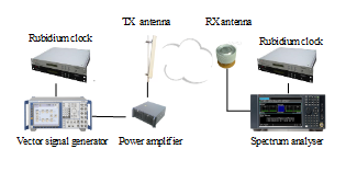Figure 1: Channel sounding system

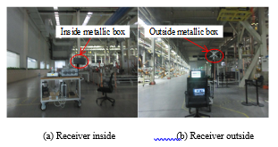Figure 2: Measurement setup

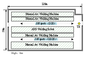Figure 3: Environment map of the automobile factory

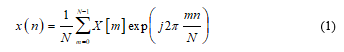
In the measurement, in order to extract the channel impulse response (CIRs), the frequency-domain method (OFDM signal) is used. There are N subcarriers in one OFDM symbol with transmitted.  denotes the excitation signal on the m-th subcarrier. The discrete time excitation signal x(n) can be given after N-point IFFT

The convolved output between the excitation signal and the time-variant CIRs denoted as a function of the discrete time variable (n) and the time delay (τ) can be expressed as

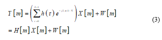
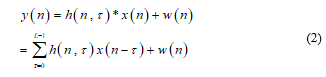where w(n) is the additive white Gaussian noise (AWGN), L denotes the amount of MPCs. In the duration of one OFDM signal, the channel is assumed as constant, i.e., h(n,τ)=h(τ). The received signals can be obtained as follows after removing the CP and FFT operation:

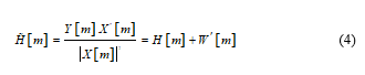
Then the frequency domain correlation processing is performed as

Finally, the extracted CIR can be obtained from (4) via the Fourier series as

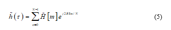Finally, the real MPCs from  can be extracted. And then the method in reference [12] is used to the noise threshold determination and path searching.

3. Results and Analysis of Measurement Data

3.1.  Path Loss Characteristics

Path loss is an important parameter, which reflects the energy loss of electromagnetic wave in the environment. Usually, previous researchs and results show that the path loss power is mainly related to the distance between the receiver and the transmitter. And when acquiring the propagation loss power and the distance between the receiver and the transmitter, path loss prediction can be described with the empirical path loss model which can be written as

where n represents the path loss coefficient, d denotes the distance in meters between the receiver and the transmitter, X_σ is the shadowing term, and A represents the intercept. The least square (LS) method is adopted to the linear fitting and estimate n in the measurement data processing. In TABLE 2, the results are listed.

Table 2: Path Loss Parameters

Frequency	LOS		OLOS
	nOus	nIns	nOus	nIns
1.1GHz	2.5	2.6	3.1	3.4
2.55GHz	2.4	2.5	3.4	3.7
5.8 GHz	2.6	–	3.2	–

The superscript Ous and Ins represent cases that the receiver antenna of the channel sounder is outside and inside of the metallic box respectively.

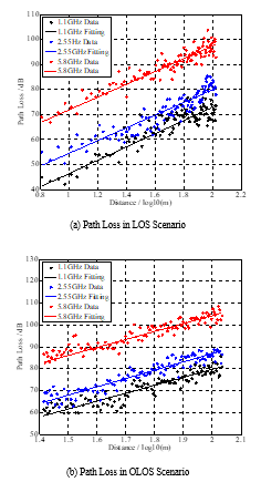Figure 4: Path Loss Exponent Extraction

Different frequency bands are measured in the same route (LOS and OLOS). The LS method is used to fit the path loss model, as shown in Figure 4, which is the situation of LOS and OLOS outside of metallic body respectively. The estimated path loss coefficient is around 2.6 in LOS, and the value in OLOS is relatively larger, around 3.2 as showed in Table 2. This is due to the fact the propagation link is semi-blocked by the metal machines and other objects. Path loss coefficient in the industrial scenarios exhibits a higher value compared to the path loss coefficient (n=2.0) in the free space model. In contrast, path loss exponent value inside metallic box is a little bit larger than the value extracted outside. This is mainly because of the energy loss of electromagnetic waves penetrating metal boxes. Moreover, it can be found that there is no clear relationship between frequency band and path loss coefficient. In reference [13] there is also similar conclusion that  path loss coefficient is independent of the frequency band. Furthermore, the results in Table 2 change significantly with the path loss coefficient acquired from different    industrial wireless channel measurements summarized in [14] (Table I). It can be assumed that the path loss coefficient varies with the environment (the position, the size, the height, and density of Metallic materials or machines in the industrial factory), links configuration and frequency. In a consequence, when planning wireless communication systems in the industrial factories, it is suggested that a larger path loss coefficient should be used.

And what’s more, according to the characteristics of the workshop in the industrial environment, under the same propagation conditions, if the receiver exists inside the large machine or inside the metallic body, a greater path loss coefficient should be selected compared to the external. Therefore, receiver location and environmental conditions in the workshop should be investigated before selecting the appropriate path loss coefficient.

3.2.  K Factor

Two different types propagation LOS and OLOS scenarios are considered in the industrial environment. The envelope of the received signal is according with Rician distribution which varies with the probability density function written as

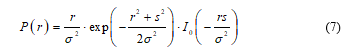where   represents the variance of the diffuse components,  is the nth-order modified Bessel function of the first kind, and  represents the power of the LOS path. A moment-based K-factor estimator is used to extract the K-factor [14]

where the closed forms of the even moment are  and , respectively.

In Table 3, K factor values of LOS and OLOS scenarios are shown. In LOS scenario, K factor values are about 5 dB, and due to metallic materials or equipments, the values in OLOS are little smaller than that in LOS scenario. Moreover, it is expected that when the center frequency increasing, the wavelength decreasing and more objects playing a role as reflectors, the K factor value decrease. Besides, K factor inside metallic body is smaller than outside. That is due to the metallic body generates additional penetration loss, so the dominant signal is attenuated. Meanwhile, the reflection scattering in the metallic body may be enhanced. This give rise to the occurrence of deep fades and yield small Rician factors.

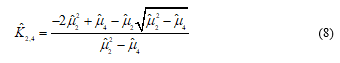
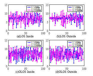Figure 5: The change of channel envelope values

Table 3: K-Factor

Frequency	LOS (dB)		OLOS(dB)
	KOus	KIns	KOus	KIns
1.1GHz	4.8	4.2	3.8	3.2
2.55GHz	5.2	4.5	4.6	2.8
5.8 GHz	7.3	–	4.3	–

The superscript Ous and Ins represent cases that the receiver antenna of the channel sounder is outside and inside of the metallic box respectively.

Figure 5 shows the channel envelope which represents the fluctuation degree of the receiving signals at different propagation scenarios (Figure 5 a, b, c, d) and the variances σ² of channel envelope in all scenarios are extracted in Table 4, which are 5.5, 3.7, 6.5, 5.6. It can be seen that when the Rx antenna is in the same environment, for example, inside of the metallic body under LOS propagation case of Figure 5(a), the envelope fluctuation of the received signals of different frequencies is basically the same. And in the same scenarios (LOS or OLOS), σ² inside metallic body is larger than outside. That means the fluctuation of signals envelope is more serious. This is because reflected and scattered waves in the metallic body are much more those outside of the metallic body. More MPCs give rise to significant fluctuation of the channel envelope and cause larger variance σ². Furthermore, it also can be found that variance σ² in OLOS scenarios is larger than that in LOS environments. This is due to the rich MPCs. These MPCs give rise to the severe fluctuation of the channel envelope.

Table 4: Variances σ² of Channel Envelope

LOS		OLOS
Ins	Ous	Ins	Ous
5.5	3.7	6.5	5.6

3.3.  Time Delay Characteristics

The time delay spread is important to digital communication system. It reflects the delay time of a multipath channel and can represent the time dispersion characteristic parameters of the channel. The statistical results are mainly the multipaths delay spread to estimate the small-scale fading of wireless channel. The RMS delay is used to quantify the parameters of the multipath channel, the following definition of RMS delay parameters is given by

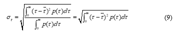where τ is time delay, p(τ) is power delay profile (PDP),  is average time delay which can be expressed as

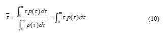
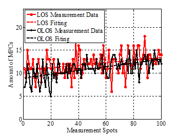Figure 6: The amount of MPCs of 5.8GHz in LOS and OLOS

In this section, the RMS delay spread values and the number of MPCs of LOS and OLOS scenarios are researched with 8 MHz bandwidth, whether it is LOS or OLOS scenario, Out or Ins condition, there is only one main path can be obtained when the excitation signal bandwidth is 0.8 MHz (corresponding to 1.1 GHz and 2.55 GHz). And more echo waves can be obtained when the excitation signal bandwidth is 8 MHz. The main reason is that when the bandwidth is 0.8 MHz, the resolvable distance of the excitation signal is 375 m, whereas, when the bandwidth is 8 MHz, the resolvable distance is 37.5 m. So, it’s much easier to make detecting MPCs when the bandwidth wider. For this reason, time delay parameters are extracted with the bandwidth in 8MHz, however, the channel envelope (not resolvable MPCs and the time delay spread) is the primary parameter extracted when the bandwidth is 0.8MHz.

Figure 6 shows the amount of MPCs of 5.8GHz in LOS and OLOS propagation conditions. It can be seen that the number of MPCs in the OLOS propagation condition is obviously more than that under the LOS propagation condition, which is mainly due to the scattered around the OLOS propagation is more abundant, and the electromagnetic waves mainly arrive at the receiving antenna by the way of reflection and diffraction. In addition, it can be seen that the number of MPCs increases slightly with the increase of distance in both LOS and OLOS propagation conditions, which is mainly due to the greater density of metal or equipment in the actual factory environment, far from the receiving end of the transmitting antenna. Meanwhile, when the bandwidth of the excitation signal is 8 MHz, the RMS results are shown in Table 5. RMS in OLOS propagation condition is larger than that in LOS, which also shows that the phenomenon of multipaths is more serious in OLOS propagation condition.

Table 5: RMS Delay Spread

Frequency	LOS	OLOS
5.8 GHz	9.37 us	15.3 us

4. Conclusions

Measurement results and analysis of the propagation fading behaviour in industrial factory environments has been presented in this paper. And two propagation types LOS and OLOS cases are considered. Particularly, special industrial propagation cases, sensors/actuators are equipped in metallic machine bodies. The results of the path loss exponent values have been reported. The estimated values are around 2.5 and 3.3 in LOS and OLOS propagation scenarios, relatively, which are larger than that of the free space model. In the research, K factor is used to described the power ratio between the direct ray and the sum of the powers of other rays. As the results shown, in LOS and OLOS scenarios, the K factor values are around 5 dB and 4 dB, respectively. And when the receiver antenna is equipped in metallic machine bodies, the path loss exponent is larger and K factor values are smaller. These are due to the metallic body generates additional penetration loss, so the dominant signal is attenuated. Further-more, channel envelope fluctuation in OLOS is more serious than LOS, and the channel envelope fluctuation inside the metallic body is more serious than outside. These are mainly because of MPCs in LOS and inside of metallic body are more abundant. What’s more, in this paper time delay parameter and the number of MPCs are researched. The RMS delay spread are 9.37us and 15.3us in LOS and OLOS scenarios. The research   results are important to the design of the IIoT for industrial scenarios.

Conflict of Interest

The authors declare no conflict of interest.

Acknowledgment

The research was supported in part by the Key Laboratory of Universal Wireless Communications (BUPT, KFKT-2018 105), Ministry of Education, P.R.China, Beijing Natural Science Foundation(NO. L172030), the Beijing Municipal Natural Science Foundation under Grant 4174102, and the Open Research Fund through the National Mobile Communications Research Laboratory, Southeast University, under Grant 2017D01 and 2018D11.

1. L. Liu, K. Zhang, C. Tao, K. Zhang, J. Zhang. “Channel measurements and characterizations for automobile factory environments.” International Conference on Advanced Communication Technology 2018:234-238. https://doi.org/10.23919/ICACT.2018.8323708
2.  S. Mumtaz, A. Alsohaily, Z. Pang, A. Rayes, K. F. Tsang, J. Rodriguez, “Massive Internet of Things for Industrial Applications: Addressing Wireless IIoT Connectivity Challenges and Ecosystem Fragmentation.” IEEE Industrial Electronics Magazine 11.1(2017):28-33. https://doi.org/10. 1109/MIE.2016.2618724
3. T. S. Rappaport, C. D. Mcgillem. “UHF fading in factories.” IEEE Journal on Selected Areas in Communications 7.1(2015):40-48..https://doi.org/10. 1109/49.16842
4. A. Miaoudakis, A. Lekkas, G. Kalivas, S. Koubias, “Radio channel characterization in industrial environments and spread spectrum modem performance.” Emerging Technologies and Factory Automation, 2005. Etfa 2005. IEEE Conference on IEEE, 2006:7 pp.-93. https://doi.org/10. 1109/ETFA.2005.1612506
5.  C. Oestges, D. Vanhoenacker-Janvier, B. Clerckx. “Channel Character-ization of Indoor Wireless Personal Area Networks.” IEEE Transactions on Antennas & Propagation 54.11(2006):3143-3150. https://doi.org/10. 1109/TAP.2006.883962
6.  E. Tanghe, W. Joseph, L. Martens, H. Capoen, K. Van Herwegen, W. Vantomme. “Large-scale fading in industrial environments at wireless communication frequencies.” Antennas and Propagation Society International Symposium, Conference IEEE, 2007. https://doi.org/10.1109 /APS.2007.4396167
7.  M. Cheffena.”Propagation Channel Characteristics of Industrial Wireless Sensor Networks.” IEEE Antennas & Propagation Magazine 58.1(2016): 66-73.https://doi.org/10.1109/MAP.2015.2501227
8.  B. Holfeld, D. Wieruch, L. Raschkowski, T. Wirth, C. Pallasch, W. Herfs, C. Brecher. “Radio channel characterization at 5.85 GHz for wireless M2M communication of industrial robots.” Wireless Communications and NETWORKING Conference IEEE, 2016. https://doi.org/10.1109/WCNC. 2016.7564890
9. J. Ferrer-Coll, P. ÄNgskog, J. Chilo, P. Stenumgaard. “Characterisation of highly absorbent and highly reflective radio wave propagation environments in industrial applications.” Communications Iet 6.15(2013): 2404-2412.https://doi.org/10.1049/iet-com.2012.0028
10.  J. Karedal, S. Wyne, P. Almers, F. Tufvesson. “Statistical analysis of the UWB channel in an industrial environment.” Vehicular Technology Conference, 2004. https://doi.org/10.1109/VETECF.2004.1399930
11. Şeyma Tütüncü, A. Kara. “UHF propagation measurements in heavy industry.” Signal Processing and Communication Application Conference IEEE, 2016.https://doi.org/10.1109/SIU.2016.7495797
12.  L. Liu, C. Tao, R. Sun, H. Chen, Z. Lin. “Non-stationary channel charact-erization for high-speed railway under viaduct scenarios.” Science Bulletin 59.35 (2014):4988-4998.https://doi.org/10.1007/s11434-0140606 -x
13.  Cheffena M. “Propagation Channel Characteristics of Industrial Wireless” IEEE Antennas & Propagation Magazine 58.1(2016): 66-73. https://doi. org/10.1109/MAP.2015.2501227
14.  Nikolic, B. Zorica “Principles of Mobile Communication : Gordon L. Stuber; Second Edition; Kluwer Academic Publishers, Boston, 2001, 752 pages, ISBN 0-7923-7998-5.” Microelectronics Journal 32.12(2001):10 50-1051.https://doi.org/10.1016/S0026-2692(01)00119-7

(Click Here)

(Click Here)