1. Introduction

This paper is an extension of work originally presented in BioSMART, the 2nd International Conference on Bio-engineering for Smart Technologies” titled ‘Biometric Database for Human Gait Recognition using Wearable Sensors and a Smartphone’ [1]. Biometrics identifiers are typical, quantifiable characters that can be used to identify and label individuals. The identifiers can be either physiological or behavioural. Physiological characteristics include, but are not limited to fingerprint, iris recognition, face recognition, retina, and palm print etc., everything related to shape of the body. Behavioural characteristics include, but are not limited to gait, voice, typing rhythm etc. They are related to pattern of behaviour of a person. Biometric identifiers are unique for each person and they can be used as a reliable means to verify identity or as a means of authentication. But collection of biometric identifiers might raise concerns about privacy and questions about how secure the collected data is. Extensive use of biometric systems has been done in different fields such as forensics for criminal identification, electronic gadgets access, human activity recognition, health status [2]. Although extensive research has been going on in the field of biometric identification and authentication for the last decade, all this has been limited to the topics of face recognition, iris recognition, voice recognition, fingerprint recognition etc. Identification of individual using their gait is an idea which is least explored and not put into practise extensively [3]. Gait recognition is defined as “automatic identification of an individual based on the style of walking” [3].  Gait is the manner in which a person walks and it is more distinctive than we realise and so a person can be identified using his walking pattern from a distance [4]. Lot of research and thought has been put into human gait recognition using floor sensors (FS), machine vision (MV) and wearable sensors (WS) [5]. Most of previous works in gait recognition were based on machine vision techniques, i.e. analysing video or a sequence of images to collect patterns. Both MV and FS based techniques have their disadvantages. MV based techniques have many interfering variables [6] and FS based technique have costly floor sensors. Recently WS using accelerometers were used for gait recognition and nowadays every smartphone has an accelerometer giving a new direction to the gait recognition researches. Our model incorporates different widely used emerging technologies in human gait recognition. Wearable sensors, and Smartphone accelerometer two such technologies. In our experiment thought has been given to various walking scenarios and other variables such as age, weight, and height.  The data acquired from the various sensors are then compared with testing data set. Different comparison methods give the matching percentage and best suited gait data. Figure 1 shows the outline of the data process that takes place in our work.

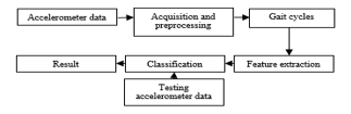Figure 1. Overall process of gait cycle signal processing

2. Methodology

2.1.  Database Collection

In a hall of 10×25 meters (indoor experiment), human gait database was collected using five wearable shimmer [7] sensor modules (integrated 3 axis MEMS accelerometer and gyroscope), and one smartphone Samsung Galaxy Note (with inbuilt NT70000 K3DH acceleration and K3G gyroscope sensors) [8], [9]. Data collected from these three techniques are saved with details like participant name, participant ID and type of walk in .dat, .csv, and .jpg formats respectively for further processing. None of the subjects has any known gait abnormalities. Figure 2 shows the overall setup for gait data collection. In this section we will talk in details about our experimental setup and collected methodologies.

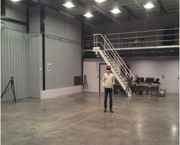Figure 2. Experimental lab used in our study

2.2.  Wearable Accelerometer and Gyroscope Sensors

From a group of 50 people comprising of 37 males and 13 females of varying age range from 14 to 52 years’ accelerometer and gyroscope data regarding gait is collected. The average age, height and weight of subjects is 26.6 years, 173.8cm and 71.2 Kg respectively. The general information regarding each subject like name, age, height, weight, and footwear are collected and kept securely for further data analysis. A walking protocol was developed and each subject were follow that protocols, which includes walking with different speeds like slow, normal and fast walk throughout the experiment. i.e. subjects should wait for 3 seconds before they start walking, then walk for a distance of four meters, then wait another 3 seconds and then walk the same distance to and fro for a duration of 45 seconds. The above same procedure was repeated for all other three types of walk.

Five wireless sensors modules (Shimmer 2r) are attached to different locations on human body like on L/R hand, L/R leg, L/R pant pocket, L/R shirt pocket and hand bag (Figure 3). The sensor locations for this study are chosen based on where a normal person carries his phone (like in pant pocket, hand, bag, upper pocket).

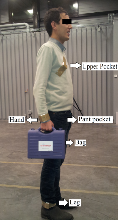Figure 3. Shimmer sensor locations

Shimmer sensor module is a small wireless sensor platform that can record and transmit physiological and kinematic data in real-time (Figure 4). Each shimmer wireless sensor has on-board microcontroller (MSP430), wireless communication via Bluetooth or 802.15.4 low power radio and local storage to micro SD card [10], [11]. The unit also has integrated 3 axis MEMS accelerometer (Free scale MMA7361) and gyroscope for motion sensing, activity monitoring and inertia measurement application. All five Shimmer sensor modules are calibrated using ‘Shimmer 9DOF Calibration application’.

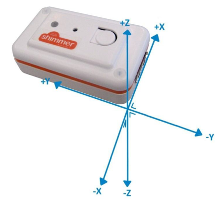Figure 4. Shimmer 2R wearable sensor

Data acquisition software named ‘Multi-Shimmer Sync’ developed by shimmer research group was used to synchronize all five shimmer modules and to transmit streamed data to PC through Bluetooth. Multi-Shimmer Sync is an application which allows for the configuration and synchronized data capture from multiple Shimmers (Figure 5) [12], [13]. All five shimmer sensor modules are configured with ±1.5g acceleration range, this range is chosen because most of the smartphone’s inbuilt accelerometers have same range. Sampling rate is set to 51.2 Hz to avoid any data transmission loss. Total data collection time for each subject is approximately 4.5 minutes. Collected data are finally stored in PC in .dat format for further processing in MATLAB.

2.3.  Smartphone accelerometer and Gyroscope

From a group of 23 subjects comprising of 16 males and 7 females of a varying age group from 21 to 39 years. The average age, height and weight of collected subjects is 27 years, 172.2cm and 72.08 Kg respectively. Smartphone Samsung galaxy note, with inbuilt NT70000 K3DH acceleration [14] and K3G gyroscope sensors are used to capture data [15]. Android application named ‘Sensor pro list’ is used to capture sensor data. Captured sensor data is then transferred to PC through Bluetooth. [16], [17]. Each subject is asked to hold the phone in hand like how they normally carry it [18]. Each subject is also asked to select the log on and log off (i.e. to start and stop) of mobile android application and walk in similar walk protocol as explained earlier [19], [20]. Table 1 shows the comparison study of database collected using two techniques.

3. Processing of Accelerometer Data

Raw data from all shimmer sensors modules is saved in DAT file format. Each subject file contains information of the five sensors. Each sensor data consists of time stamp, accelerometer

(in x, y, and z axis) and gyroscope (in x, y, and z axis). similarly, smartphone data is a saved in CSV file format. Each subject smartphone sensor data also consists of time stamp, accelerometer (in x, y, and z axis) and gyroscope (in x, y and z axis).

3.1.  Data Preprocessing

• Data reading

The data reading procedure is divided into three steps.  In first step, each participant data such as name, ID, height, weight, gender, age, sensor location is read one by one which are stored in excel file. In second step, sensor data files of each participant are read from assigned folders and subfolders for creation of gait data base features. Finally, all data files are exported to MatLab and headers of each file are read to identify each subject recorded

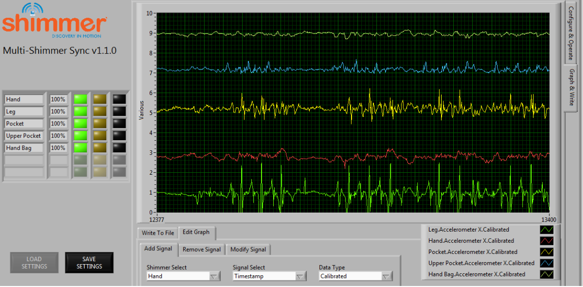Figure 5. Sample gait data collection with Multi shimmer sync software

Table 1. Comparison of the two techniques

	Wearable Shimmer sensor	Smartphone
Sensor specification	Five Shimmer 2r’s with inbuilt 3-axis MEMS Freescale MMA 7361 accelerometer	One Samsung Galaxy Note  (inbuilt  K3DH acceleration & K3G gyroscope sensors)
Computer interface	Bluetooth	Bluetooth
Software used	Multi Shimmer Sync	Sensor Pro list
Range of sensor	+/-1.5 g	+/-1.5 g
Sensor sampling frequency	51.5 Hz
Location of sensor	Leg, Hand wrist, pant pocket, Shirt pocket and bag (left and right side)	Hand
Number of participants	50(37 male, 13 female)	23 (16 male, 7 female)
Range of age	14 to 52 years	21 to 39 years
Mean of age	26.6 years	27
Range of height	150-193 cm	154-189 cm
Mean height	173.8 cm	172.2 cm
Range of weight	50 to 107 kg	50 to 105 kg
Mean weight	71.2 kg	72.08 kg

sensor data belong to which sensor location (like leg data\hand data\pocket data etc.) and to which data such as accelerometer, gyroscope and time stamp values. Since each sensor at different body location has different processing techniques such as data recorded from leg is entirely different from data recorded from pocket; therefore, data each particular sensor is identified and processed with techniques explained below. Processing methods also depends on the sensors used for data collection, like sampling frequency of sensor, location of sensor. Effective preprocessing techniques improve recognition rate. Figure 6 shows a flow chart of data processing of testing and training data.

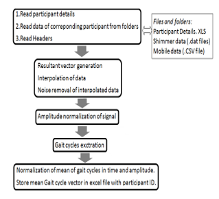Figure 6. Flow chart of data processing of testing and training data

• Data processing

Resultant vector: The output from various accelerometers data will vary depending on how the shimmer sensor modules are oriented and also all three different axes have varying moments. To overcome this problem, the resultant vector (xyz) of the accelerometer in X, Y, and Z axis output is calculated using Euclidean norm as given in (1). The first three plots of Figure 7 shows X, Y, Z plots. The last plot in Figure 7 shows the resultant vector of all axes.

Interpolation: Raw accelerometer data has irregular periodic intervals therefore interpolation is needed to have data samples at regular intervals.  Interpolation [21] is a method of constructing new data points within the range of a discrete set of known data points. Many interpolation methods like linear, polynomial, spline interpolation methods can be used. In our work, spline interpolation of period 10 m sec is used. Spline interpolation [22] uses low-degree polynomials in each of the intervals, and chooses the polynomial pieces such that they fit smoothly together [23].

Noise removal: Weighted moving average (WMA) method is applied to our interpolated data to remove unwanted noise from the signal. This method is fast and easy to implement. In WMA method, the nearest neighbors are more important than those more away, while in other methods all the neighbors have equal weight. The formula for WMA with a sliding window of size 5 is given in (2).

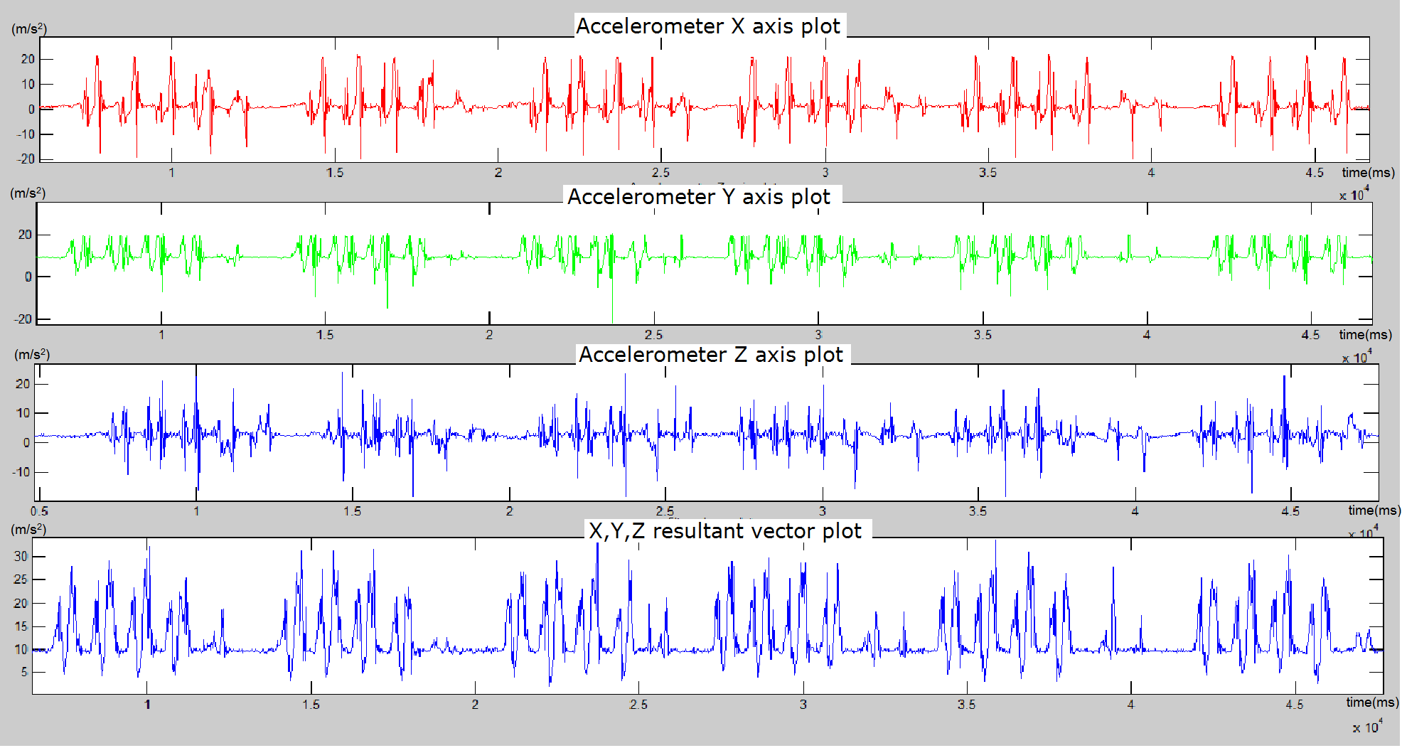Figure 7. Unprocessed raw gait signals

where:  is the acceleration value at position t

Amplitude Normalization: For easy computations, raw accelerometer data is normalized from 0 to 1 as shown in Figure 8 by applying (3)

Where: newsi – amplitude normalized signal

             xyzif – interpolated and filtered signal of accelerometer resultant vector signal

                 mi – minimum range of sensor

                  ma – maximum range of sensor

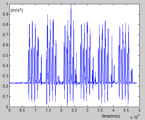Figure 8. Amplitude normalization of whole gait signal

• Gait cycles extraction and Time Normalization

Cycle Detection: A gait cycle will comprise of two footsteps and it is detected by finding the minimum points in a given cycle.  The end of the preceding one will mark the start of each cycle up to final cycle of the gait signal. Fake minimum points are eliminated by calculating mean cycle time and standard deviation. If a gait cycle has a cycle length which falls outside of the mean time ± standard deviation is considered to be as fake cycles and will be eliminated. Since all sensors collect gait data whose minimum points should mark the start of another gait cycle, the gait detection algorithm will work for all the sensors used. In Figure 9, the first plot shows extracted gait cycles from an amplitude normalized signal. Cycle length as well as mean length of all gait cycles are estimated and saved as feature vectors. There are chances that the length of each gait cycle might vary from cycle to cycle; therefore, normalization of signal in time is needed. Gait cycles are normalized to 1 second duration. Here 1 second is chosen as a random standard value. Figure 9 shows difference between normalized and un-normalized gait cycles.

In some cases, after time normalization also fake cycles are observed, so again these fake cycles are eliminated by calculating trimmed mean cycle (TM cycle). TM cycle is calculated by calculating mean and standard deviation (SD) of all gait cycles and if point lies beyond ±SD of mean cycle then that particular cycles eliminated. Figure 10 shows a normalized trimmed gait cycle.

• Normalization of Mean gait

After elimination of fake cycles, Mean cycle, Median cycle and Trimmed mean cycle are calculated to represent a gait cycle feature vectors. Mean cycle refers to the time domain waveform at which each time sample represents the mean cycle value over a fixed time window of the gait cycle length. Median cycle refers to the time domain waveform at which each time sample represents the median cycle value over a fixed time window of the gait cycle length. Mean, Median and TM gait cycle which is normalized in time (for 100 samples) and in amplitude (0 to 1 range) is then stored in an array of 100 values are stored in Microsoft excel.

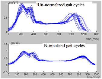Figure 9. Un-Normalized and Normalized gait cycles

Since each sensor at different body location has different processing techniques such as data recorded from leg is entirely different from data recorded from pocket; therefore, each sensor is identified and processed with techniques explained below. Processing of different sensors varies in cutoff and in elimination of fake cycles techniques.

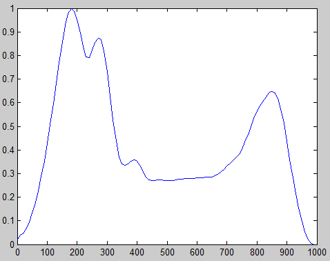Figure 10. Normalized Trimmed Mean Gait Cycle

3.2.  Elimination of fake cycles

Before calculating average gait cycle fake cycles can be eliminated by using following techniques:

1. By calculating mean cycle length(MCL) and standard deviation (SD) of all identified cycles. Cycle length falling beyond MCL ± SD are eliminated.
2. By calculating trimmed mean(TM) cycle of all cycles. TM cycle is obtained by calculating mean of cycle points which lie in between Mean cycle point ± SD of cycle point and cycle points which lie beyond range are eliminated.
3. By matching maximum point of all gait cycles i.e. by calculating mean gait cycle and searching maximum point of each cycle around SD of mean gait cycle maximum point.

3.3.  Data analysis for obtaining results

This section explains how data has been analysed for obtaining results.

• Analyzing methods

This sub section explains the calculation of gait biometric system performance  metrics like FAR,FRR,EER,TRR and FRR [24]. The performance metrics are calculated by creating Distance score tables and explained below.

Distance score table calculation:  Obtained average gait cycles for all subjects for different walks(SW, NW, FW) at different sensor location for both smartphone data and wearable data are compared against each other. Distance metrics like Manhatten  and Euclidean methods are used and explained below:

Manhatten distance: This is also known as absolute distance and the formula is shown in (4). Manhattan distance between two points is the sum of the absolute difference in their Cartesian coordinates. In addition, this distance metric is the computationally least expensive one.

Hamming distance: Hamming distance is utilized to detect and correct errors in digital communication. Hamming distance between two data are said to be the least number of changes that could make both the data same. For example, the hamming distance between ‘name” and ‘meme” is 2 and between 337895 and 235817 is 4.

Euclidean distance: This is a slight modification of the Manhattan distance, see (5). Instead of taking the sum of the absolute differences we now take the square root of the sum of all differences squared.

    From distance metric methods a score tables are generated. Valid subject has a less distance score as compared to not valid subjects. Distance score table is classified into accepted and rejected matches based on classifier cutoff. Classifier cutoff is choosen from percentage of maximum score value from score table. Accepted matches again have two cases like Genuine Accepted Match (GAM) and Fraud Accepted Match (FAM). GAM is accepted match of correct subject i.e. accepted match is of correct subject and is recognized by classifier. FAM is counted when a false match is accepted and recognized as correct match. Similarly rejected matches have two cases like Genuine Rejected Match (GRM) and Fraud Rejected Match (FRM). GRM is genuine match is supposed to be accepted but is not recognized. FRM is counted when false match is accepted and recognized as an incorrect match. FRM is fraudulent match is supposed to be accepted but is recognized as incorrect.

Biometric matrices like False acceptance rate (FAR), false reject rate (FRR), Total recognition rate (TRR), Genuine recognition rate (GRR) and Equal error rate (ERR) are calculated from generated score table and are explained as below.

False acceptance rate (FAR) is a measure of how precisely biometric data can be compared and recognized (6). It represents the chance that the comparison will accept a wrong input as an affirmative match. The input is not supposed to match with the template data but invariably the system considers this match to be correct. FAR is calculated by testing known biometric templates against a huge collection of data.

False rejection rate (FRR) is a measure of the chance that the system will wrongly reject a genuine input as a match that doesn’t fit (7).

EER is the value at which FRR and FAR are equal and is obtained by plotting graph between FAR and FRR. TRR and GRR are calculated using (8) and (9). In TRR number of recognized samples is sum of genuine accepted and fraud rejected samples but GRR is calculated only for genuine accepted samples.

Where N is the total number of comparison samples.

     For data collected from wearable sensor for 50 subjects, two files for each of three different walking scenarios (SW, NW and FW) we have total 300 (50*3*2) gait features for one sensor location. So total of 100 gait features of each scenario (e.g. for normal walk sensor at leg have 100 templates) are compared against each other and with other scenario i.e. comparison with walks like slow-slow(S-S), normal-normal (N-N), fast-fast (F-F), slow-normal(S-N), slow –fast(S-F), normal-fast (N-F).  In comparison of same sensor location and same walk there are five cases, there are case 0: don’t count (DC), case 1: GAM, case 2: GRM, case 3: FAM, case 4: FRM. DC case is when comparing two similar files because each subject has two files when we compare first file of a subject to the first file of subject it is obvious match. So this case is not counted for metric calculation. Also if there is match between first file of subject to second file this is counted in GAM. So cases 0, 2, 3 are not valid (error matches), FAR and FRR are calculated using FAM and GRM respectively. In comparison with other different walks like), slow-normal(S-N), slow –fast(S-F), normal-fast (N-F) case 0 (DC) will not be there.

    Table 2 shows the FAR, FRR, TRR and GRR values with different classifier cutoffs. Consider FW-FW comparison with cutoff 40%, it has FAR of 2.92% which says that 2.92 subjects out of 100 subjects are falsely accepted, FRR of 0.07% means 0.07 subjects which are genuine are rejected, TRR of 97.01% says how efficiently a classifier can classify matches correctly whether it is genuine accepted match or fraud rejected match and GRR of 93% represent the ability of classifier to identify genuine accepted matches. From Table 2, as cutoff percentage increases GRR increases at the cost of increase in sum of errors (FAR+FRR). So classifier cutoff is chosen such a way by having tradeoff between GRR and errors.

Table 2. Pocket hamming method results

100 samples	Classifier Cut-off=10%	Classifier Cut-off=20%	Classifier Cut-off=30%	Classifier Cut-off=40%	Classifier Cut-off=50%
Pocket	FAR  FRR  TRR%  GRR	FAR  FRR  TRR%  GRR	FAR  FRR  TRR%  GRR	FAR  FRR  TRR%  GRR	FAR  FRR  TRR%  GRR
S-S	0             0.67   99.3300   33.00	0.72    0.3900   98.8900   61.00	3.0800    0.2200   96.7000   78.00	6.2900    0.1200   93.5900   88.00	8.4500    0.0300   91.5200   97.00
s-n	2.3300    1.55   96.1200   22.50	7.30    1.0800   91.6200   46.00	12.9800    0.8500   86.1700   57.50	17.9900    0.6500   81.3600   67.50	20.4500    0.5300   79.0200   73.50
s-f	1.9700    1.77   96.2600   11.50	10.88    1.3200   87.80   34.00	23.6700    0.9100   75.4200   54.50	31.4400    0.6900   67.8700   65.50	34.3100    0.6000   65.0900   70.00
n-n	0.1800    0.22   99.6000   78.00	0.93    0.0800   98.99   92.00	1.8800    0.0500   98.0700   95.00	2.4800    0.0200   97.5000   98.00	3.0600    0.0200   96.9200   98.0000
n-f	5.5000    1.03   93.4700   48.50	12.77    0.6500   86.58   67.50	15.1800    0.5800   84.2400   71.00	17.9300    0.5100   81.5600   74.50	19.1300    0.4700   80.4000   76.50
f-f	0.0500    0.50   99.4500   50.00	0.63    0.1500   99.22   85.00	1.8800    0.0900   98.0300   91.00	2.9200    0.0700   97.0100   93.00	3.9100    0.0400   96.0500   96.00

4. Results

    Figures 11 and 12 shows the recognition rate of all wearable sensors using Hamming method of classification.    Figures 13 and 14 shows the recognition rate of all wearable sensors using Manhattan method of classification Same sensor to sensor walk (like S-S, N-N, F-F) comparison have highest recognition rate value than comparison with other walks (S-N, S-F, N-F). In Figures 11,12,13 and 14 shows that Manhattan classifier has better classification results than Hamming method. Sensor located at Pocket and Leg has highest recognition rate than other sensor location. Results in table shows the EER value of different sensors. The EER values ranges from 0.21 to 2.258. Same sensor to sensor walk EER values (for S-S, N-N, F-F) comparison have less error values than comparison with other walks (S-N, S-F, N-F). EER rate of F-F comparison is more than S-S and N-N because when a subject is asked to walk fast, walk becomes unstable. Also among all six scenarios S-F comparison has highest EER as there is template mismatching and comparison between stable (SW) and unstable walk (FW) gives higher EER.

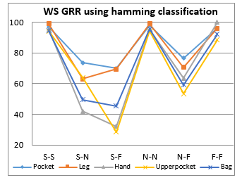Figure 11. Wearable sensors GRR values using hamming method

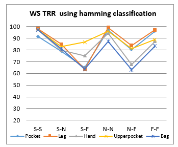Figure 12. Wearable sensors TRR values using hamming method

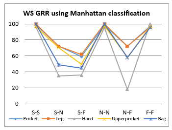Figure 13. Wearable sensors GRR values using Manhattan method.

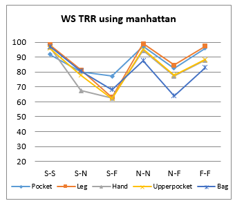Figure 14. Wearable sensors TRR values using Manhattan method

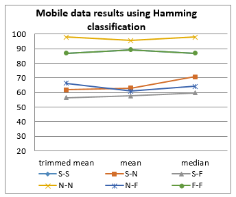Figure 15. Mobile data results of Hamming method

Table 3. EER table of Hamming and Manhattan tables

	Hamming					Manhattan
	Pocket	Leg	Hand	Upper Pocket	Bag	Pocket	Leg	Hand	Upper Pocket	Bag
S-S	0.44	0.2700	0.3245	0.3786	0.3874	0.4400	0.2700	0.3245	0.3786	0.3616
s-n	1.6200	1.6000	1.9605	1.3521	1.7691	1.6100	1.6100	2.2445	1.3386	1.7562
s-f	1.7900	1.9200	2.2039	2.0146	2.1436	1.7800	1.8900	2.2580	2.0687	2.1823
nn	0.2100	0.1700	0.4867	0.4056	0.8781	0.1900	0.1700	0.4867	0.4056	0.8781
n-f	1.3600	1.5000	2.0822	2.0416	2.0919	1.4600	1.5000	2.2715	2.0416	2.0919
f-f	0.2400	0.2600	0.5949	0.6760	0.8910	0.2300	0.2600	0.6084	0.6760	0.8910

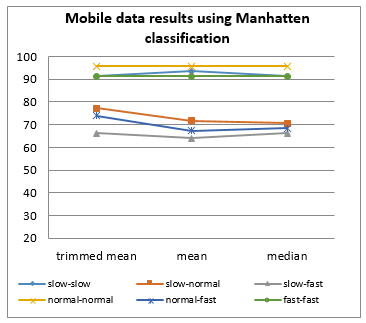Figure 16. Mobile data results of Manhattan method

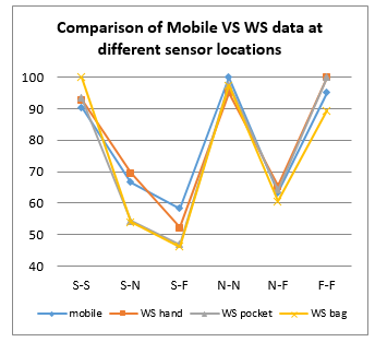Figure 17. Comparison of mobile data results with wearable sensors location like hand, pocket and bag data

    Figures 15,16 shows the results of Manhattan and Hamming methods for six different walk scenarios for which comparisons are done TM, mean and median cycles respectively. Table 3 shows the EER values, whose range is from 1.2287 to 4.0643. EER values of mobile data are more than wearable sensors data.

In real life people hold\place their phones in different location on body such as (pocket, hand, suit case etc…). Figure 17 shows the comparison results of GRR for 23 participants’ data of mobile, wearable sensors at hand, pocket and bag. Even though mobile data have more or same wearable sensors recognition rates, mobile data has more EER values. Smartphone’s have accelerometers that are good enough to detect human gait with slight modification on their frequency range and sensitivity of sensor. Although investigations are going on extensively in this field of research, an attempt to include comparison of different techniques and that to taking into account different walking scenarios was never seen before. This paper will give insight into how different walking posters will affect the gait recognition of different sensors.

Table 4. Mobile data EER rate

	Hamming			Manhattan
	Trimmed mean	Mean	Median	Trimmed mean	Mean	Median
S-S	1.6068	1.7013	1.6068	1.6068	1.6068	1.6068
s-n	3.5917	3.6389	3.5444	3.5917	3.6389	3.5444
s-f	4.0643	4.0643	4.0170	4.0643	4.0643	4.0170
n-n	1.7486	1.7958	1.7958	1.6541	1.7486	1.7013
n-f	3.5917	3.6389	3.3554	3.5917	3.6389	3.3081
f-f	1.3233	1.2287	1.3233	1.2287	1.2287	1.2760

Human gait is affected by many factors, and changes in the normal gait pattern can be transient or permanent. The factors can be of various types:

• Extrinsic: Several extrinsic factors such as terrain, footwear, clothing, cargo(luggage).
• Intrinsic: Intrinsic factors are sex (male and female), weight, height, age, etc.
• Physical: Physical factors such is the weight, height, physique
• Psychological: Psychological factors are the type of personality, emotions
• Physiological: When talking about is physiological anthropometric characteristics
• Pathologic, pathological factors can be for example trauma, neurological diseases, musculoskeletal, psychiatric disorders
• Intrinsic factors such as age, height and weight are also analyzed in our work.

   The entire sample was divided into three equal groups as shown in Figure 18 for comparing wearable sensors for different weight range. And it was found that the average TRR for range of 50 to 58 Kg is more than other two ranges.

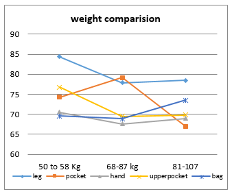Figure 18. Average GRR (of six scenarios) value of wearable sensor data comparison for different weights range

For sensors located at leg, pocket and hand the average GRR value falls with increase in age group, while for sensors located at upper pocket and bag, the GRR value doesn’t follow any trend. In general, average recognition rate decreases as age increases, which has been explained by Richard W. Bohannon [25] in his work. Many other physiological factors like brain stability, thoughts etc. changes as age increases (Figure 20). Weight and height factors are studied as shown in Figure 18 and Figure 19 respectively. Different walks had different energy of signal which can be used for activity recognition. Even though three walks have different energies, they have more or less same gait features in common.

5. Conclusion

Our future work needs to give emphasis to increasing the number of participants in the experiment to about 120-150 because the number of participants affect the calculated recognition rate by a great deal and helps in making the calculations accurate. Time elapsed and activity recognition are some other factors that will have to be pondered over. This research will provide us with an idea of how changes in subject’s daily routine affect the rate of recognition. How a person walks can vary depending on different parameters such as footwear, type of clothing, with or without luggage, walking surface and terrain, human factors; thus the above mentioned issues needs to be looked into further. Our research needs to be further extended to include other types walking patterns including running, climbing stairs up/down, jumping and sitting. The smartphone data used in the study was exclusive to one smartphone and one data processing software. More work is to be done on this part. Data from different smartphones having a variety of built in accelerometers and using some other data processing software. Effect of Gait difference of same height subjects with different weight and effect of load are also to be studied further. Insight was also provided on how other co parameters affect the gait recognition of the sensors.

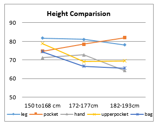Figure 19. Average GRR (of six scenarios) value of wearable sensor data comparison for different heights range

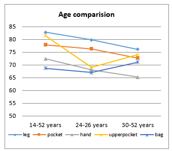Figure 20. Average GRR (of six scenarios) value of wearable sensor data comparison for different weights range

Conflict of Interest

The authors declare no conflict of interest.

Acknowledgment

This work was supported by Haute-Normandie Region as part of The Nomad Biometric Authentication (NOBA) project.

1.  S. K. A. Kork, I. Gowthami, X. Savatier, T. Beyrouthy, J. A. Korbane and S. Roshdi, “Biometric database for human gait recognition using wearable sensors and a smartphone,” 2017 2nd International Conference on Bio-engineering for Smart Technologies (BioSMART), Paris, 2017, pp. 1-4
2.  Qian Cheng, Yanen Li_, Joshua Juen, “Classifier of Gait Pattern for Detecting Abnormal Health Status”, SenSys’12Toronto, ACM 978-1-4503-1169-4, Canada 2012.
3.  D. Hodgins, “The Importance of Measuring Human Gait,” European Medical Device Technology, 2008.. F Sayegh, F Fadhli, F Karam, M BoAbbas, F Mahmeed, JA Korbane, S AlKork, T Beyrouthy “A wearable rehabilitation device for paralysis,” 2017 2nd International Conference on Bio-engineering for Smart Technologies (BioSMART), Paris, 2017, pp.1-4.
4.  Mark Ruane Dawson, “Gait Recognition”,(technical report) Department of Computing Imperial College of Science, Technology & Medicine London 2002.
5.  Q. Meng b, B. Li a, H. Holstein, “Recognition of human periodic movements from unstructured information using a motion-based frequency domain approach,” Volume 24, Issue 8, Pages 795–809, Department of Computer Science, University of Wales, August 2006.
6.  T. Massart, C. Meuter and V. B. Laurent, “On the complexity of partial order trace model checking, Inform. Process,” 2008.
7.  M. Davis and H. Putnam, “A computing procedure for quantification theory.,” in Journal of ACM, 1960
8.  E. Abraham, S. Alkork, F. Amirouche, E. Hande, S. P. Rai and S. Biafora, “Experimental Investigation of Posterior Elbow Dislocation in a Primate Model,” 2007 29th Annual International Conference of the IEEE Engineering in Medicine and Biology Society, Lyon, 2007, pp. 5099-5102
9.  Al Kork S, Amirouche F, Abraham E, Gonzalez M. Development of 3D Finite Element Model of Human Elbow to Study Elbow Dislocation and Instability. ASME. Summer Bioengineering Conference, ASME 2009 Summer Bioengineering Conference, Parts A and B ():625-626
10.  S. Said, S. AlKork, T. Beyrouthy and M. F. Abdrabbo, “Wearable bio-sensors bracelet for driver as health emergency detection,” 2017 2nd International Conference on Bio-engineering for Smart Technologies (BioSmart), Paris, 2017, pp. 1-4.
11.  F Sayegh, F Fadhli, F Karam, M BoAbbas, F Mahmeed, JA Korbane, S AlKork, T Beyrouthy “A wearable rehabilitation device for paralysis,” 2017 2nd International Conference on Bio-engineering for Smart Technologies (BioSMART), Paris, 2017, pp.1-4.
12.  Ho, N. S. K., Tong, K. Y., Hu, X. L., Fung, K. L., Wei, X. J., Rong, W., & Susanto, E. A. (2011, June). An EMG-driven exoskeleton hand robotic training device on chronic stroke subjects: task training system for stroke rehabilitation. In 2011 IEEE
13.  Taha Beyrouthy, Samer Al. Kork, J. Korbane, M. Abouelela, “EEG Mind Controlled Smart Prosthetic Arm – A Comprehensive Study”, Advances in Science, Technology and Engineering Systems Journal, vol. 2, no. 3, pp. 891-899 (2017).
14.  “http://www.shimmer-research.com.,” [Online].
15.  Sung-Jung Cho, Eunseok Choi, Won-Chul Bang, Jing Yang, “Two-stage Recognition of Raw Acceleration Signals for 3-D Gesture-Understanding Cell Phones,” Tenth International Workshop on Frontiers in Handwriting Recognition 2006.
16.  M. O. Derawi, “Accelerometer-Based Gait Analysis A survey,” in NISK conference., 2010.
17.  Mohammad Omar Derawi, “Accelerometer-Based Gait Analysis A survey,” pp 33-44, NISK-2010 conference.
18.  Tobias Stockinger, “ Implicit Authentication on Mobile Devices,” Ubiquitous Computing, Media Informatics Advanced Seminar LMU, Summer Term 2011(Tech Report), University of Munich, Germany 2011.
19.  Jani Mäntyjärvi, Mikko Lindholm, “Identifying Users of Portable Devices from Gait Pattern with Accelerometers,” pp. ii/973 – ii/976 Vol. 2, IEEE 2005.
20.  Yuzuru Itoh, Manabu Miyamoto, “Convenient use of Accelerometer for Gait Analysis,” pp 21-31, Bulletin of the Osaka Medical College, 2008
21.  M. Lindholm and J. Mäntyjärvi, “Identifying Users of Portable Devices from Gait Pattern with Accelerometers,” IEEE, vol. Vol 2, pp. 973-976, 2005.
22.  S.-J. Cho, E. Choi, W.-C. Bang and J. Yang, “Two-stage Recognition of Raw Acceleration Signals for 3-D Gesture-Understanding Cell Phones,” in Tenth International Workshop on Frontiers in Handwriting Recognition, 2006.
23.  Jordan Frank, Shie Mannor, “Activity and Gait Recognition with Time-Delay Embeddings,” Twenty-Fourth AAAI Conference on Artificial Intelligence 2010.
24.  Martin Hynes, Han Wang, “Off-the-Shelf Mobile Handset Environments for Deploying Accelerometer based Gait and Activity Analysis Algorithms,” Engineering in Medicine and Biology Society, pp. 5187 – 5190, IEEE 2009.
25.  R. W. Bohannon, “Comfortable and maximum walking speed of adults aged 20—79 years: reference values and determinants,” 1997.

(Click Here)

(Click Here)