1.Introduction

Ultrasound imaging is the most commonly-used nonivasive real-time diagnostic tool in clinical applications because of its free of radiation and ease of use [1]. However, traditional ultrasound devices are bulky because of the large amount of digital data that needs to be simultaneously processed. For greater operational convenience, low power hand-held devices have come into prominence [2–4]. To minimize the size of ultrasound imaging systems, research laboratories continue to propose approaches based on modern signal and image processing methods. Their intent is to improve the image quality and diagnostic accuracy, without human body and measuring the blood flow in vessels through Doppler shift [6].

A number of approaches have been reported for ultrasound imaging using both linear array and phased array [7–11]. One-dimensional ultrasound transducer arrays are used to get 2D images, and two-dimensional transducer arrays have been applied to produce 3D ultrasound images [12–14]. The ultrasound produces images through the backscattering of the mechanical energy from boundaries through tissues. Because of this property, a 1D image could be produced by 1 transducer element exciting ultrasound waves along a straight line, called scanline (SL), and a 2D image could be generated by repeating the same step for all transducer elements. With a frame rate of approximately 30 fps, ultrasound imaging is considered to be a real-time imaging technique. However, the relatively poor soft tissue contrast limits the performance of ultrasound imaging technique. In addition, the increase in integration density tends to increase the power consumption, which is a major constraint in the implementation of digital signal processing (DSP) architectures especially for hand-held ultrasound imaging system. Although some ultrasound devices are implemented based on application-specific integrated circuits (ASICs) to reduce cost and power consumption [15], the ASIC-based design is not preferred by researchers due to its inflexibility for advanced applications. On the contrary, FPGA, because of its reconfigurability, has become an ideal alternative to ASIC. There are some existing FPGA based designs on ultrasound, but these designs are limited by several criteria discussed below.

First, it is hard to implement the DSP portion of the system with a low hardware complexity, while not impacting the spatial and temporal resolutions of the system. In fact, portable ultrasound imaging systems are limited by the low resolution and high power consumption. Increased number of transducer elements, though providing higher resolution, making the entire data rate at ADC interface reach a forbidding level that challenges not only the power consumption but also the data transmission ability. In addition, such large transducer array requires hugh analog-front-end (AFE) and digital circuitry operates in parallel, such as lownoise-amplifier (LNA), time-gain controller (TGC), and analog-to-digital converter (ADC). However, the large number of hardware duplication may cause a lot of implementation issues when integrated into portable form factors, including heat dissipation, crosstalk interface, I/O packaging. Several prior methods have been developed to reduce hardware complexity. A 64 channel power-efficient architectures version without the real time controller (RTC) has been shown by [16]. Other schemes described the DSP algorithms used in digital beamforming [17–19]. In addition, an ASICbased programmable ultrasound image processor is shown by [20]. A 16-channel FPGA-based real-time high frequency digital ultrasound beamformer is discussed by [21], but it could only support 30 fps frame rate, which constrains the image quality.

Seconds, the temporal resolution is bounded by the bandwidth of the ultrasound imaging system, which is limited by the ADC implementation [22,23]. The temporal resolution in digital beamforming systems can typically be improved in two ways: either using phase rotation, also known as direct sampled inphase/quadrature (DSIQ) beamforming, or through interpolation-based filtering. However, phase rotation degrades image quality as it assumes the ultrasound signal to be a narrow band [4,24], and interpolationbased filtering requires up-sampling before low-pass filtering, which requires the operation of the DSP portion on high frequencies, and therefore raises the energy cost. Therefore, we need to improve the methods above to reduce power consumption.

Third, applying exact delays on corresponding signals is a challenge, because the amount of delay between two subsequent sampled signals may vary based on the nature of dynamic beamforming. An iterative algorithm for calculating delay information in real-time has been implemented by [25]. However, the delay resolution in that system is bounded by the frequency of the delay calculation module. Therefore, a higher operating frequency is necessary to acquire more accurate delay information. Another widely used method is precomputing the delays. However, to overcome the impending memory limitation of FPGAs, only a pseudodynamic focusing technique is utilized where delay information is only updated for a pre-determined depth rather than for a pre-determined delay resolution [26]. Different articles introduced the digital beamformer design using a 5 MHz center frequency beamformer linear array implemented on FPGA as discussed by [27] and with a 50 MHz center frequency annular array by [28,29]. A research-aimed FPGA-based digital transmit beamformer system for generating simultaneous arbitrary waveforms has been developed by [30]. Others have applied over sampling techniques and single transmit focusing as other methodologies for digital beamforming [31].

Therefore, there is a need to develop resourcefriendly, power-efficient, and space-efficient architectures and methods for both properly delaying sampled signals and correctly acquiring delay information for a portable ultrasound device, where innovative designs of AFE and mixed-signal interface are keys to the next generation portable ultrasound devices. State-of-theart portable ultrasound typically operates at 2 to 4 MHz with less than 64 active transducer elements.

In this paper, we present our 128-channel portable ultrasound imaging system embedded in an Arria V FPGA (Altera Inc., San Jose, CA, USA), where several methods are introduced, such as polyphase filter, memory management block, and active aperture, with which we resolve the issues discussed above so as to deliver a resource friendly ultrasound imaging system. Our ultrasound imaging system, compared to prevailing 32-channel [26] and 64-channel ultrasound imaging system [32], outputs higher resolution images with the better use of FPGA area. An overview architecture block diagram of the developed N-channel power-efficient and space-efficient ultrasound imaging system is shown in Figure 1. For the AFE part, a serial low voltage differential signaling (LVDS) interface protocol is used to get a fast analog acquisition, which serves as a serial way to recover parallel data. In addition, the echo-backed signal on each channel is amplified by a TGC amplifier to compensate for signal attenuation through propagation in the medium. The TGC amplifier is implemented on the AFE part as shown in Figure 2. The AFE implementation is out of the scope of this paper and will not be discussed in detail. The delay-and-sum (DAS) module in the mid end processing module receives the compressed timing information and outputs beamformed signal without decompression.

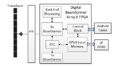Figure 1: Architecture block diagram of the ultrasound digital beamformer based on a single FPGA.

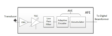Figure 2: AFE architecture block diagram in the ultrasound digital beamforming system.

2. System Architecture

Figure 3 shows the detail of the beamforming architecture of the N-channel FPGA-based ultrasound imaging system. The midend beamformer will first pass the signal to S2P module to parallel the signal, since the AFE will serialize 2 signals from neighboring channels. Then, each signal will be passed into a coarse delay module, which delays the signal from the corresponding channel by integer numbers of the sampling period, T_s. The signal is then passed into a fine delay module, which delays the signal from coarse delay module by a fraction of T_s, and an apodization weight module, which multiplies the signal by a weight window function. The coarse delay block is achieved through controlling the writing process to the first-in-first-out (FIFO) memory to get valid data. The fine delay block is employed to replace the traditional way of optimizing the resource and is accomplished by a polyphase FIR filter. Finally, the processed signals from the N channels will be summed and sent to the backend processing module. The back end processing module processes acquired data based on an user-defined imaging mode, which can be selected via the Android tablet. The FPGA local memory is connected with an external memory, LP DDR3 to store the large amount of pre-computed delay information. The architecture of the ultrasound imaging system supports apodization and dynamic focusing, and is able to achieve a high-performance imaging system. In the following subsections, we will present the architecture of the Tx and Rx beamformer, the implementation of the midend processing module, the backend processing module, the control signal generation, and the calculation of the propagation delay.

2.1. AFE Architecture

AFE contains an LNA, an LVDS interface protocol, a TGC amplifier, and a low-pass filter, as shown in Figure 2. The LNA is used for amplifying small echoed back signals; LVDS interface protocol is used for getting a fast analog acquisition; the low-pass filter is used for cutting off the high-frequency noises. Inside the AVE, an adaptive encoder and an accumulator is employed. The accumulator detects transition edge of each piecewise-constant section and calculate the length. The adaptive encoder module performs adaptive thresholding and converts the amplitude variation into ternary timing information. The adaptive encoder consists of a comparator and a threshold generator. Two 1-bit ADCs are with in the comparator, and each receives input of the input signal and a low-threshold or a high-threshold signal, generated by the threshold generator. The comparator will outputs +1 or -1 if the input signal is greater than the high threshold or low than the low-threshold, respectively, and then requires the threshold generator to update the comparison parameter for the next comparison based on the input variation; otherwise, the comparator simply outputs 0. In this way, unit amplitude +1 or -1 could be assigned without loss of generality.

Some modulation methods, including the time encoding machine (TEM) [33], delta modulation [34], and integrate-and-fire scheme [35], converts amplitude information into timing information, and both TEM and delta modulation include a negative feedback loop to lock the input signal. In addition, these techniques will force the entire circuit keeps on flip-flopping, similar to a sigma-delta modulator output with constant input, and firing all the time even when there is no input signal. Also, typical integrate-and-fire scheme calculates the running average and also fires even when no variation occurs, resulting in unnecessary power overhead. Whereas in our adaptive encoder, the circuits fire only when significant variation occurs. As a result, the proposed adaptive encoder modulates the amplitude variations into delay information more efficiently.

2.2. Tx and Rx Architecture

The Tx beamformer supports 128 channel ultrasound beamforming signals, formed by two essential parameters: pulse-shape, assumed to be the same for all channels, and channel-delay, the value of which may vary among channels, and some channels could even be disabled. The two parameters are inputs to SPI ports, governed by the SPI clock. The SPI clock may run at different frequency compared to Tx clock which provides the Tx delay granularity.

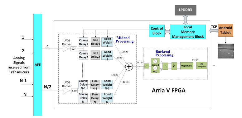Figure 3: Architecture of ultrasound receiver of the single FPGA-based the ultrasound digital beamformer, showing the midend processing and the backend processing module with the control block and the local memory management block.

Figure 4 shows the architecture of Rx beamformer, which receives control signals from both RTC and local memory management block, which will be discussed in section 2.5, and outputs control signals to AFE. Eight sub-blocks made up the frame of the Rx block, and each comprises an LVDS receiver, a Frame Align module, a data management block, and a FIFO memory block. The Rx AFE SPI module outputs control signals serially.

2.3. Mid end Processing Architecture

The core of mid end processing module is coarse delay filters and find delay filters. The coarse delay filter delays the signals by the integer number multiplication of the sampling period, T_s. This block is implemented as a FIFO buffer. The coarse delay outputs a buffered signal when the desired control delay equals to the number of signals stored in the FIFO buffer. In the dynamic beamforming, some signals are used twice for the alignment. It is satisfied by this mechanism. As a result, if the control signal is greater or equal to the number of signal in the FIFO buffer, it is possible that when the control signal increment by 1, the coarse delay output remains the same. Hence, to get the same sampled signal, the coarse delay should be incremented by one as well, which prevents updating output signals. Therefore, by focusing the points from the nearest to the farthest along a scanline, the desired delays for all channels increase simultaneously.

Fine delay filter delays signals by a fraction of the sampling period, T_s. Figure 5 shows the architecture of the fine delay filter. As shown in Figure 5, the fine delay filter uses 48 FIR low-pass filters, from C0 to C47. Their parameters are calculated based on the baseband width and the carrier frequency. The 48 filters are grouped into 8 taps, with 6 phase coefficients per tap. Each set serves to multiply the input signals, or buffered signals, by the corresponding coefficients.

Then, the multiplied signals are summed up to produce the interpolation signals.

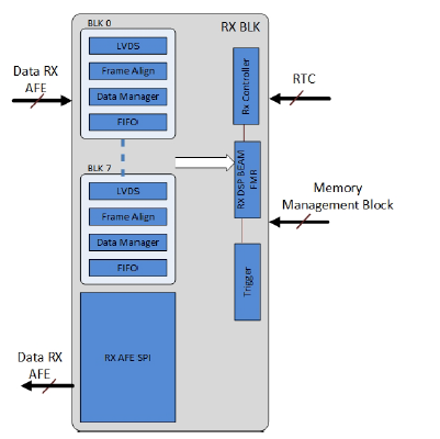Figure 4: The Rx block diagram, showing Rx block is controlled by the control signal and RTC, and contains several sub blocks 8 LVDS blocks, 8 frame align blocks, 8 data management blocks, and 8 FIFO memory blocks.

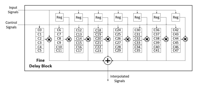Figure 5: Block diagram of poly-phase fine delay filter with 7 registers for rejecting the last repeat signals and 8

Based on the desired phase shift, the control signals generated by the control block select which set of coefficients will be used to multiply the input signals. The purpose of using register buffer is to reject the last repeated signals, because it is possible that when the coarse delay increases by 1 the output of coarse delay × 6 low-pass filters for interpolation.

blocks are not updated. Therefore, the clock-gating scheme is introduced to prevent such hazard. Once the coarse delay is increased by 1, the pipeline enable signal will be pulled down to gate the clock. Therefore, the pipeline in the fine delay block will be stalled in one cycle to reject data input.

2.4. Backend Processing Architecture

Figure 3 also shows the architecture of the backend processing module. The backend processing module includesa high-pass filter, a demodulator, a numerically controlled oscillator (NCO), and a low-pass filter. The parameters of demodulation block are determined using Matlab (TheMathwork’s Inc., Natwick, MA, USA). The data in this block is beamformed in 2 steps: before quadrature demodulation and after quadrature demodulation. The first step is the high pass filtering followed by the low pass filtering. This allows users to define filter option through the Android GUI. The second step architecture contains a down-sampling block, a magnitude I/Q demodulation block, and a log compression block. The I/Q demodulation block is used to extract the amplitude from the compressed data and outputs the interpolated data, where I and Q are 12 bits signed signal. The magnitude calculator outputs I² + Q², a 23-bit value. The log compression block is used to compress the data by taking its natural log value, which reduces the dynamic range, and outputs a 8-bit value.

2.5. Control Signals Generation

Control signals are generated by 2 blocks: RTC and the control block. Figure 6 is an overview of RTC. RTC contains 2 major blocks: the memory and RTC finite state machine (FSM). RTC FSM generate control signals based on data loaded from memory and controls Tx and Rx block along with memory.

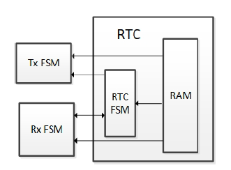Figure 6: RTC block diagram showing the how RTC communicates with Tx and Rx block.

All N datapathes in Figure 3 are controlled by the control block. The control block generates control signals based on information passed from the local memory management block, where the FPGA local memory locates. An external memory is used to accommodate the FPGA local memory to store the large amount of pre-computed delay information. The corresponding delay information will be loaded into FPGA local memory based on the imaging mode that is selected on the user side, and the command will be sent wirelessly to the control block. The control block controls all delay filters by loading pre-computed data stored in the FPGA local memory. The FPGA local memory updates itself by reading data from an external memory. However, since it takes much more time to retrieve data from the external memory than from the local memory, it is necessary to adjust the data load process, necessitating the memory management block. Figure 7 shows the architecture of the memory management block. The FPGA local memory receives data from the external memory. The input data is passed into a demux, which is controlled by the number of scanlines processed. Each demux output is connected to half of the FPGA local memory, the output of which is connected to a mux, which is controlled by the number of scanlines processed. The output of the mux is the output of this block. Local memory A and B are used as buffers, where A is used to buffer the current scanline and B is used to buffer the next scanline. The demux will pass input data to local memory A if the number of scanline processed is an odd number, and to B otherwise, represented by 2k + 1 and 2k, respectively, where k is a non-negative integer. The mux will output data from local memory A if the number of scanline processed is an even number, and from local memory B otherwise. With this technique, the FPGA local memory is always passing the current scanline data and next scanline data, reducing the time spent on transferring data from the external memory to the control block.

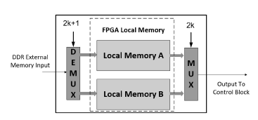Figure 7: Block diagram of local memory management system for control signal generation process.

3. Propagation Delay Calculation

Beamforming is a algorithm which takes inputs from the transducer elements and outputs the summed signals. The implementation of beamforming algorithms is one of the deterministic factors in the ultrasound imaging quality [36]. In this paper, a delay-and-sum beamformer is used, because of its high accuracy on close-range beamforming, which is a dominant in medical ultrasound systems. Several focusing techniques have been developed for delay-and-sum beamforming, including the fixed focusing, dynamic focusing, and composite focusing techniques. The composite focusing technique is simply a special case of dynamic focusing [37] and will not be discussed in this paper.

Figure 8 shows how the signals alignment system

(SAS) works. As Figure 8 presents, the signals echoed back from the focal point reach different channels at different time, which causes delay. The SAS module is used to align the signals and then pass them into the summer, which outputs the summed signal.

The difference between dynamic focusing and fixed focusing is that dynamic focusing requires the focal point to be continuously changed. Dynamic focusing could extend the field depth without satisfying the frame rate [38]. Therefore, the dynamic focusing technique is used when the SAS operates in the receive phase, and the delays of all channels are adjusted, because of the requirement of dynamic focusing. Figure 9 demonstrates the changes in the signals’ flight paths during the receive phase. In Figure 9, multiple channels are used to receive ultrasound signals. Focal points on the same scanline are under detection. By assuming the scanline begins from the position of channel A, we can determine the focal points of the signals sampled by channel A. There exists a depth in the physical positions between every two sampled data points which is clearly evident in Figure 9. The distance, d, between two focal points, P₁ and P₂, satisfies that d ≈ (c ×T_s)/2, given that d is small enough. Here, c is the average ultrasound speed in human body.

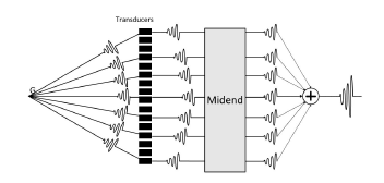Figure 8: Signals alignment in ultrasound digital beamforming system.

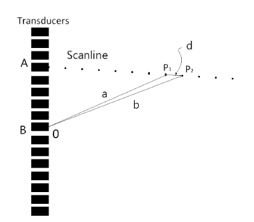Figure 9: Variations of echo paths in receiving signals used in dynamic focusing technique.

Now, the signals that are variably received by the transducer elements should be delayed using dynamic beamforming. For the focal point P₁ in Figure 9, it is assumed that the time interval between transmission and reception by channel A is T₁. The time interval for channel B to receive it is T₂, where T₂ > T₁. Consequently, a delay of (T₂−T₁) in the signal echoed back from P₁ is observed to be aligned with the signal in channel B. For the subsequent focal point P₂, the time that corresponding signals are received by Channel A and Channel B, Tˆ₁,Tˆ₂ respectively, are:

According to the property of the triangle, we have

b −a < d, where a is the distance between P₁ and channel B, and b is the distance between P₂ and channel B. Thus it is derived that:

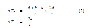It implies that the corresponding signal of P₂ has arrived at channel B before its next sampling. We can retrieve the fraction delay between two samples after sampling the next signals in channel B provided that ∆T₁−∆T₂ is relatively short. But if we get a large enough ∆T₁−∆T₂, the corresponding signal has to be accessed without sampling the next signal. Here, we use the previous sampled signal from channel B twice and align with both signals received from the channel for P₁ and P₂. The resolution our system can support is λ/16. There are techniques that use a 100 MHz sampling rate with digital interpolation filters [21], which allow the signals to be sampled at a lower frequency and concurrently get more precise delays [39,40].

The delay values are pre-computed and pre-loaded to the external memory, as mentioned in the previous section.

4. System Specifications

The T_x firing frequency, also called pulse repetition interval (PRI), is constrained by several theoretical limitations: the round trip delay (RTD), the wireless backhaul limitation (WBL), and the DDR to FPGA interface limitation.

First, P RI is given by:

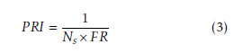where N_s refers to the number of samples per scanline, and FR is the frame rate of the system. N_s could be calculated by:

N_s = f_s ×RT D    (4) where f_s indicates the ADC sampling rate, as de-

fined previously, and RT D is calculated by 5,

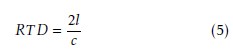where l is the penetration depth. The penetration depth varies among different mediums. Theoretical time for penetration depth is shown in Table 1: WBL is given by

where N_b is the number of bits per sample; and W_b, the wireless bachhaul speed, is determined by the device employed. The WBL indicates the lower bound for P RI.

Table 1: Theoretical RTD for Different Penetration Depth.

Depth of Penetration (cm)	RTD (µs)
9	116.88
7	90.10
5	64.94
3	38.96

5. Dynamic Power Management

To reduce power consumption, we modified the traditional B-mode imaging to perform the following scans: for each focal point on a specific scanline, excite a pulse from the transducer corresponding to that scanline, and receive signals with all transducers within active aperture. Repeat this procedure for all scanlines. The reason this method is able to reduce power consumption and conserves the image quality is because of 7:

where F_n is the f-number, a fixed number for one transducer, f is the focal depth and D is the diameter of the hypothesis aperture. According to 7, the maximum hypothesis aperture size is proportional to the depth of the furthest focal point, which indicates that channels outside the hypothesis aperture does not help the preservation of image quality. Figure 10 shows how this equation helps reduce the power consumption. As shown in Figure 10, for focal point B, the hypothesis aperture is the black region in the center. When focal point B is processed, all transducers outside the hypothesis aperture could be turned off. When the focal point is changed from B to A, the size of the hypothesis aperture increases, so more channels could be turned on to receive signals. The transducers in the white region are still off, because they are outside the hypothesis aperture for focal point A.

To further reduce power consumption, we consider turning off additional transducer elements with negligible image quality degradation. The idea is to choose a range of transducer elements, the range of which is called limited aperture, shown in Figure 11, and listen from the transducer elements within the limited aperture. However, there are cases where the transducers are not enough to cover the whole limited aperture, as illustrated in Figure 12. In this case, the aperture covering both transducers and limited aperture is called active aperture, and only the channels within the active aperture are turned on.

To get better image quality, the received signal for a focal point is the sum of all signals received by different active transducer elements. This can be achieved by a simple transducer elements shift operation shown in Figure 13. When processing SL₁, the transducer elements within the active aperture only are turned; for SL₂, the limited aperture is shifted down by 1 transducer element, so that one more transducer element is turned on to receive signals; and when SL_n is processed, all transducer elements within the limited aperture are turned on. This shift operation will last until all scanlines are processed.

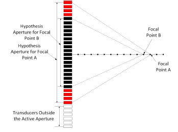Figure 10: Hypothesis aperture for different focal points on one scanline, showing the variation of hypothesis aperture with the change of focal depth.

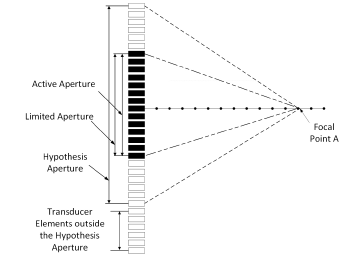Figure 11: Limited aperture size for further focal points showing the relationship between active aperture, limited aperture, and hypothesis aperture in the normal case.

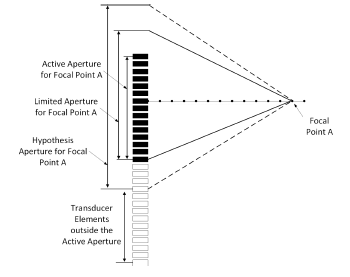Figure 12: Limited aperture size for further focal points showing the relationship between active aperture, limited aperture, and hypothesis aperture when the transducer elements cannot cover the whole limited aperture.

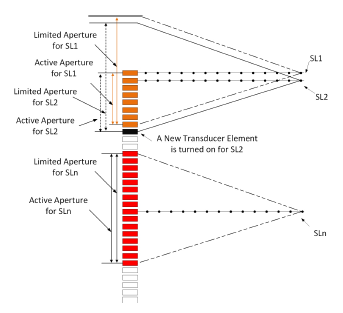Figure 13: Transducer elements shift operation illustration. The limited aperture will be shifted based on the location of scanlines.

For a 128-channel ultrasound system, the maximum hypothesis aperture size could reach up to 256, including a virtual array consisting of 128 elements (the intersection between hypothesis aperture and aperture out of limited aperture) and physical aperture consisting of 128 elements. To observe the degradation on performance, different sizes of the limited aperture are used to receive echoed back signals. The corresponding images are shown in Figure 14. These images show that with the receive aperture increasing, a higher imaging contrast resolution could be achieved. When the limited aperture is larger than half of the effective aperture (the whole transducer array), the degradation is conceptually negligible. With the aperture size less than half of the effective aperture, most parts of the image such as blood vessels could still be clearly imaged. However, the bright spots are spread around. Hence, when the aperture size increases, a better signal-to-noise ratio (SNR) is achieved. To acquire a good measurement of the degradation, the formula below is applied to quantitatively check the difference among those images.

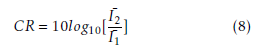where CR is the contrast ratio, and I¯₁,I¯₂ are the average intensities in the region of interest and the region of reference, respectively. This provides a quantitative assessment of the performance of contrast restoration, the result of which is shown in Table 2.

As we discussed above, we know that the image quality will vary depending on the active aperture size. Thus, for the case we illustrated, we could merely keep the 128-channel aperture instead of the 256-channel aperture. Therefore, based on the analysis above, we could turn off all transducers outside the active aperture to reduce power consumption, while still conserving the image quality.

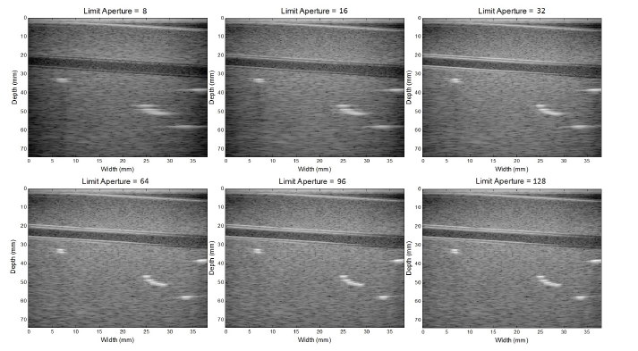Figure 14: Ultrasound images generated with different limited aperture size chosen, showing that the image quality reserves when the limited aperture size is greater than or equal to half of the effective aperture.

Table 2: Contrast Ratio of the Images with Different Limited Aperture Values. Aperture 128 96 64 32 16 8 CR 16.3842 16.0634 15.4241 14.7033 14.637 14.637

To estimate the power consumption, we assume that each transducer element could be independently switched “on” and “off” by using power-gating technology. For a linear array, the power consumption is approximately proportional to the total number of active elements used during scanning one frame:

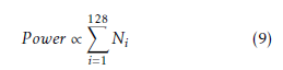where N_i is the number of data channels used for the i^th scanline. N_i could be represented by

where Ch_right and Ch_{lef t} are the indexes of right most and left most active transducer element, respectively. They can be represented as in 11 and 12.

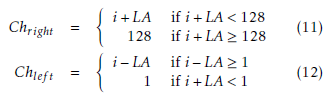where LA is the size of limited aperture. The index of the very right channel is on the right of the channel which is in the position of the current scanline. The limitation of aperture allows the channels whose index is larger than i +LA/2 to be turned off. If the very right channel outside the zone of the transducer, i.e. whose index is larger than 128. The 128^th channel will be the right bound.

According to 9, the normalized power consumption for different aperture limitations are calculated and plotted in Figure 15. With negligible degradation, the 128-channel ultrasound device will consume 75% of the power that the all-channel effort devices consume.

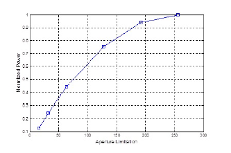Figure 15: Normalized power consumption for different limitations of aperture.

6. Results and Discussion

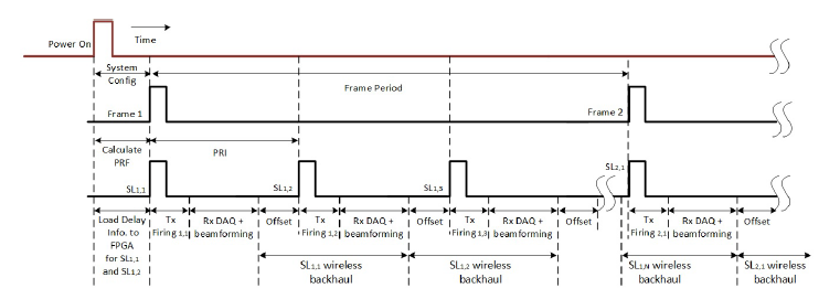Figure 16: PRI adjustability based on system requirements, showing the conceptual timing of the single-FPGA-

The timing of the beamforming architecture is shown in Figure 16. Initially, the system is powered up, allowing switching mode power supplies (SMPSs), AFE ICs, FPGA, and wireless to be on. When the user selects the smart probe function via tablet GUI, a data packet containing initial system configuration is sent to the RTC wirelessly. The RTC will extract the imaging mode, application, array type, FR, Ns, and number of scanlines (NSL) from this packet. Then the RTC will continue to based ultrasound imaging system.

load and send delay information for SL₁ and SL₂ into Rx beamformer using the mechanism described in section 2.5. The delay information for SL₁ in frame 1 will also be loaded into the T_x beamformer inside the 128channel Tx AFE (in Figure 16, SL_a,_b indicates the b^th scanline in the a^th frame). This configuration time is pre-determined, and this allows the Tx beamformer to send a “Ready” signal to the RTC. Upon receiving the signal, the RTC initiates the Tx pulse firing by sending pulse-in, pulse-enable, and scan-enable signals. After Tx firing, the Rx beamformer begins to listen and beamform received signals. The data is sampled based on the ADC sample rate. DDR3 control data has already been preloaded into FPGA local memory for SL₁, so this is applied to the coarse delay for beamforming. The I/Q data is then backhauled throught the PCIe solution based wireless module. Notice there is a gap named “Offset” in Figure 16. This offset time is used when the R_x beamformer sends beamformed data to the display device and the T_x beamformer receives the 3 signals (pulse-in, pulse-enable, and scan-enable) from the RTC. This offset time is the reason why the WBL is the lower bound for PRI, as mentioned in section 4.

The program on Android device, once the system starting up, will wirelessly send the pre-calculated delay information to the probe, which will send the Android device the digitized data pack during the wireless backhaul after applying the information and beamforming. Upon receiving the package, the program will create an image and apply a filter on it. The filtered image will finally be displayed.

The dynamic power management approach allows power reduction on a high end system with higher channel count and operating at higher supply voltages. The approach allows dynamic control of the AFE operational state based on the ultrasonic pulse repetition frequency (PRF). The PRF of an ultrasonic smart probe is dictated primarily by the speed of its wireless backhaul. Regardless of the depth of penetration, there is going to be a sizable offset after the successful reception of the furthest received signal, and the beginning of the next transmit firing. This offset region, as has been discussed above, is where the receiver is sitting in an idle state and burning DC power. Hence, we would prefer to turn off the most power inefficient regions of the receiver.

Our ultrasound imaging system supports 40 MHz

ADC sample rate (25 ns temporal resolution) with 12 MHz max fundamental frequency and 80% bandwidth.

Also, a max pass band of 16.8 MHz is available with 20 dB rejection. For the fine delay filter, each filter is implemented based on 48 FIR filter, which has 0.2 dB ripple and 20 dB rejection. The PRI we used is 200 µs with FR of 39 fps for 128-channels, limited by RTD of 65 µs at penetration depth of 5 cm, and a WBL of 180 µs (N_b = 12 bits/sample, W_b = 140 MHz). The TDL of 51.2 µs, constrained by the bus speed of 40 MHz. The digital beamformer is implemented with register-transfer level (RTL) in Verilog and synthesized by Quartus II (Altera Inc., San Jose, CA, USA) for Altera Arria V. The flow chart of the RTC is shown in Figure

17. The Android GUI program has been developed with C++ to control the system. All the control signals were generated in the tablet and are transferred wirelessly to the prototype board after the user configures the required input data via the tablet.

To improve the utilization of memory, a deltacoding scheme is used. From the previous mechanism, we know that the coarse delay for each channel monotonously increases and the maximum difference of coarse delay signals between two focal points for each channel is one. One bit is enough to be used as the delta between two coarse control signals. The absolute values of coarse delays for the first focal point are given at the beginning of scanning a line. The delays change according to the delta value. The fine delay has 3 bits, which are updated every sample. Therefore, there are 4 bits to be stored for each sample and each channel. Figure 18 shows the data organization in local memory. The memory is updated every scanline. The beginning 9 bits are used for initial absolute coarse delay. Subsequent 3 bits are used to indicate the fractional delay for the first focal point. Following 4-bit words are used to update delay information, whose first bit is the increment of coarse delay and other 3 bits are the fractional delay.

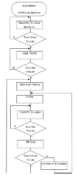Figure 17: Flow chart of the real time controller for the ultrasound digital beamformer.

The system provides 128-channels of transmitter channels with a maximum of 32 excited pulses while simultaneously receiving signals at a 40 MHz sampling rate and converting them to a 12-bit binary number. The digitized data from all channels are first fed through the processor in the FPGA, and then stored in LPDDR3 memories by using direct memory access. These raw data are accessed by the beamforming processor to build the image that will be sent to the Android device wirelessly for further processing.

Figure 19 shows the finite state machine (FSM) used to coordinate the data flow of the local memory to dynamically generate the control signals (Coarse Delays and Fine Delays). Since there is limited bandwidth between the receiver and the memory, we introduced the scheme to dynamically change delays to accommodate the dynamic beamforming. To do that, last-level local memory is used on the receiver, which is 16×4×9 large for 16 channels. The memory is organized so that each channel has 4 × 9 bits in the local memory. Initially, those memories are filled by 4×9 bits of data, so that the initial fine delays and fraction delays are known (This is done in the first 4 status S0, S1, S4, S5). Once those 4 statuses are set, the delays can be initialized. Then the delays are held until the receiver starts working (state S2). As the receiver starts receiving data, the delays change. The new delay information (4 bits, 1 for coarse delay change, 3 for new fine delay) is sent into the control blocks in each cycle. In this phase, the local memory needs to keep updating data (S3 does this). When the counter hits the length of the scanline depth, one scanline is done. It then reverts to the initial state.

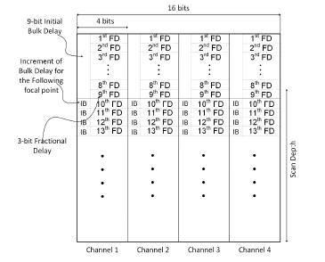Figure 18: Flow chart of the real time controller for the ultrasound digital beamformer.

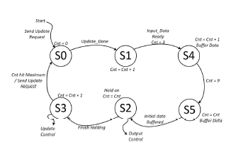Figure 19: Finite state machine for generating the control signal for the ultrasound digital beamformer based on a single FPGA.

The beamformer that applies delays to the echoes of each channel is implemented by the strategy that combines coarse and fine delays (4 ns). This system is capable of achieving a maximum frame rate of 50 fps; this is mainly limited by the maximum speed we can achieve while wirelessly backhauling the data to the Android device. Table 3 shows the device utilization for the whole architecture, mid-end and the control block. The 128-channel model consumes 130,547 adaptive logic modules (ALMs), the beamforming block consumes

128,044 ALMs, and the control section consumes 2,147 ALMs. The designed board contains the architecture in FPGA and DDR3, which is the external memory to store all delay information. We use the FPGA Mezzanine Card (FMC) connector to feed testing data into FPGA from stimulus boards. The board wirelessly backhauls the ultrasound image for display on a tablet or smart phone as shown in Figure 20(a).

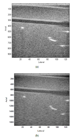Figure 20: Ultrasound images displayed on tablet processed by (a) single Altera Arria V FPGA based ultrasound digital imaging system and (b) Simulink.

To validate our design, another FPGA is added for testing purposes: the beamformed data is stored temporarily in the added FPGA and will be sent to the Android device after testing. A software-based beamformer is simulated by Matlab and Simulink. Data generated by a quantized Matlab module is used to verify the output of the board, as shown in Figure 20(b). The sum operation across all channels is pipelined to incorporate numerous inputs and process them at a high clock frequency. The first stage in the pipeline contains 64-inputs, each producing the sum of the incoming 12-bits from 2 channels. The resulting 32 outputs are summed in pairs in the second pipeline stage. The last summation stage is truncated to a 12-bit number and fed into the high pass filter. The image is generated from a Verasonics machine (Vantage 128, Verasonics Inc., Kirkland, WA, USA).

Table 3: Implementation Parameters

Parameter	Value	Percentage
ALMs	130,547	96
Registers	41,450	–
Pins	263	40
Block memory bits	2,754,067	18
PLLs	3	8
DLLs	1	25

7. Conclusion

In this paper, we present a series of techniques: interpolation filter, limited aperture size and dynamic power management to improve the efficiency of a fully dynamic ultrasound beamformer for a handhold real time 128-channel ultrasound system, providing higher image resolution compared to the 32-channel [26] and 64-channel beamformer [32]. The proposed architecture is programmed and synthesized in a single Arria V FPGA using Verilog, allowing fully dynamic beamforming in a low-cost single FPGA implementation. This proposed digital beamformer can be used in generic ultrasound imaging systems, personal portable ultrasound health care, as well as the cart ultrasound machine. It is useful for portable low-power ultrasound and high performance ultrasound imaging with the genuine support of dynamic beamforming, while most current ultrasound devices employ pseudo dynamic beamforming. In addition, the power consumption and hardware utilization was reduced by a huge amount.

1.  J. A. Jensen, “Medical ultrasound imaging,” Progress in Biophysics and Molecular Biology, vol. 93, pp. 153-165, no.1, 2007.
2.  J. J. Hwang, J. Quistgaard, J. Souquet, and L. A. Crum, “Portable ultrasound device for battle field trauma,” in Proc. IEEE Ultrason. Symp., vol. 2, pp. 1663-1667, 1998.
3.  M. Karaman, P. c. li, and M. odonnell, “Synthetic aperture imaging for small scale systems,” IEEE Trans. Ultrason. Ferroelectr. Freq. Control, vol. 42, no. 3, pp. 429-442, 1995.
4.  C. Yoon, J. Lee, Y.M. Yoo, T.-K. Song, “Display pixel based focusing using multi-order sampling for medical ultrasound imaging,”, 3rd ed. Electronics Letters, vol. 45, no.25, pp. 1292- 1294, Dec. 3, 2009.
5. A. Assef, J. Maia, E. Costa “A flexible multichannel FPGA and PC-based ultrasound system for medical imaging research: initial phantom experiments,” Research on Biomedical Engineering, vol. 31, pp. 277-281, Sept. 2015.
6.  A. Murtaza, D. Magee, and U. Dasgupta. “Signal processing overview of ultrasound systems for medical imaging,” SPRAB12, Texas Instruments, Nov. 2008.
7.  J. A. Jensen, O. Holm, L. J. Jensen, H. Bendsen, H. M. Pedersen, K. Salomonsen, J. Hansen, and S. Nikolov, “Experimental ultrasound system for real time synthetic imaging,” IEEE Ultrasonics Symp, pp. 1595-1599, 1999.
8.  M. O’Donnell, M. J. Eberle, D. N. Stephens, J. L. Litzza, B. M. Shapo, J. R. Crowe, C. D. Choi, J. J. Chen, D. W. M. Muller, J. A. Kovach, R. J. Lederman, R. C. Ziegenbein, K. San Vicente, and D. Bleam, “Catheter arrays: can intravascular ultrasound make a difference in managing coronary artery disease,” IEEE Ultrasonics Symp, pp. 1251-1254, 1997.
9.  J. Schulze-Clewing, M. J. Eberle and D. N. Stephens, “Miniaturized circular array,” IEEE Ultrasonics Symp, pp. 1253-1254, 2000.
10.  J. P. Stitt, R. L. Tutwiler and K. K. Shung, “An improved focal zone high-frequency ultrasound analog beamformer,” IEEE Ultrasonics Symp, pp. 617-620, 2002.
11.  C. Dusa, P. Rajalakshmi, S. Puli, U. B. Desai and S. N. Merchant, “Low complex, programmable FPGA based 8-channel ultrasound transmitter for medical imaging researches,” in 2014 IEEE 16th International Conference on e-Health Networking, Applications and Services (Healthcom), Natal, 2014, pp. 252-256.
12.  A. Bhuyan etal:, “Integrated circuits for volumetrix ultrasound imaging with 2-D CMUT arrays,” IEEE Trans. Biomed. Circuits Syst., vol. 7, pp. 796-804, Dec. 2013.
13.  J. W. Choe, O. Oralkan, and P. T. Khuri-yakub, “Design optimization for a 2-D sparse transducer array for 3-D ultrasound imaging,” Proc. IEEE Ultrason. Sysmp., 2010, pp. 1928-1931.
14.  J. Song etal:, “Reconfigurable 2D cMUT-ASIC arrays for 3D ultrasound image,” Proc. SPIE Meidcal Imaging, vol. 8320, p. 83201A, Feb. 2012.
15.  V. S. Gierenz, R. Schwann,T .G. Noll, “A low power digital beamformer for handheld ultrasound systems,” in Solid- State Circuits Conference, Proceedings of the 27th European, pp. 261-264, 18-20 Sept, 2001.
16.  M. Almekkawy , J. Xu and M. Chirala, “An optimized ultrasound digital beamformer with dynamic focusing implemented on FPGA,” in 36th Annual International Conference of the IEEE Engineering in Medicine and Biology Society, Aug 26, pp. 3296-3299, 2014.
17.  C. Fritsch, M. Parrilla, T. Sanchez, O. Martinez, “Beamforming with a reduced sampling rate,” IEEE Ultrasonics, vol. 40, pp. 599-604, 2002.
18.  S. R. Freeman, M. K. Quick, M. A. Morin, R. C. Anderson, C. S. Desilets, T. E. Linnenbrink, and M. ODonnell, “Delta sigma oversampled ultrasound beamformer with dynamic delays,” IEEE Trans. Ultrason., Ferroelect., Freq. Contr., vol. 46, pp. 320- 332, 1999.
19.  M. Kozak and M. Karaman, “Digital phased array beamforming using single-bit delta-sigma conversion with non-uniform oversampling,” IEEE Trans. Ultrason., Ferroelect., Freq. Contr., vol. 48, pp. 922-931, 2001.
20.  C. Basoglu, R. Managuli, G. York, and Y. Kim, “Computing requirements of modern medical diagnostic ultrasound machines,” Parallel Computing, vol. 24, pp. 1407-1431, 1998.
21.  C. H. Hu, X. C. Xu, J. M. Cannata, J. T. Yen and K. K. Shung, “Development of a real time high frequency ultrasound digital beamformer for high frequency linear array transducers,” IEEE Trans. Ultrason., Ferroelect., Freq. Contr., vol. 53, no. 2, pp. 317-323, 2006.
22.  D. K. Peterson and G. S. Kino, “Real-time digital image reconstruction: A description of imaging hardware and an analysis of quantaization errors,” IEEE Trans. Sonics Ultrason, vol. SU-31, pp. 337-351, 1984.
23.  B. D. Steinberg, “Digital Beamforming in ultrasound,” IEEE Trans. Ultrason., Ferroelect., Freq. Contr., vol. 39, no. 2, pp. 716-721, 1992.
24.  H. Sohn, S. Seo, J. Kim and T. Song, “Software implementation of ultrasound beamforming using ADSP-TS201 DSPs,” Proceedings of SPIE, vol. 6920, pp. 69200Z-69200Z-11, 2008.
25.  H. T. Feldkamper, R. Schwann, V. Gierenz, T.G. Noll, “Low power delay calculation for digital beamforming in handheld ultrasound systems,” IEEE Ultrasonics Symposium, vol. 2, no., pp. 1763-1766, Oct 2000.
26.  Gi-duck Kim, Changhan Yoon, Sang-Bum Kye, Youngbae Lee, Jeeun Kang, Yangmo Yoo, Tai-Kyong Song, “A single FPGAbased portable ultrasound imaging system for point-of-care applications,” IEEE Trans. Ultrason., Ferroelect., Freq. Contr., vol. 59, no. 7, pp. 1386-1394, July 2012.
27.  B. Tomov and J. A. Jensen, “A new architecture for a single chip multi-channel beamformer based on a standard FPGA,” IEEE Ultrasonic Symp., pp. 1529-1533, 2001.
28.  P. J. Cao and K. K. Shung, “Design of a real time digital beamformer for a 50 MHz annular array transducer,” IEEE Ultrasonic Symp., pp. 1619-1622, 2002.
29.  P. J. Cao,C. H. Hu and K. K. Shung, “Devolepment of a real time digital high frequency annular array ultrasound imaging system,” IEEE Ultrasonics Symp, pp. 1867-1870, 2003.
30.  A. A. Assef, J.M. Maia, F.K. Scheneider, E.T. Costa, V.L. Button, “A programmable FPGA-based 8-channel arbitrary waveform generator for medical ultrasound research activities,” in Engineering in Medicine and Biology Society (EMBC), 2012 Annual International Conference of the IEEE, vol., no., pp. 515-518, Aug. 28 2012-Sept. 1, 2012.
31.  M. A. Hassan, and Y. M. Kadah, “Digital signal processing methodologies for conventional digital medical ultrasound imaging system,” American Journal of Biomedical Engineering, vol. 3,no. 1, pp. 14-30, 2013.
32.  C. Hu, L. Zhang, J. M. Cannata, J. Yen, K. K. Shung, “Development of a 64 channel ultrasonic high frequency linear array imaging system,” Ultrasonics, vol. 51, no. 8, pp. 953-959, 2013.
33.  A. A. Lazar and L. T. Toth, “Perfect recovery and sensitivity analysis of time encoded bandlimited signals,” IEEE Trans. Circuits Systems 1, vol. 51, no. 10, pp. 2060-2073, Oct. 2004.
34.  N. S. Jayant and A. E. Rosenberg “The preference of slope overload to granularity in the delta modulation of speech,” Bell System Technical Journal, vol. 50, no. 10, Dec. 1971.
35.  A. S. Alvarado and J. C. Principle, “From compressive to adaptive sampling of neural and ECG recordings,” in Proc. of IEEE Int. Conf. on Acoustics, Speech, and Signal Processing (ICASSP), pp. 633-636, Apr. 2011.
36.  J. Lu, H. Zou, and J. F. Greenleaf, “Biomedical ultrasound beam forming,” Ultrasound in Med. and Biol., vol. 20, pp. 403-428, 1994.
37.  H. Yao, “Synthetic aperture methods for medical ultrasonic imaging,”, Ph.D. thesis, Univ. of Oslo, Norwa, 1997.
38.  I. LIE, M. E. TANASE, D. LASCU, and M. LASCU, “Ultrasonic beamforming with delta-sigma modulators,” in Proc. of the 10th WSEAS International Conference on CIRCUITS, 2006, pp. 344-349.
39.  R. A. Mucci, “A comparison of efficient beamforming algorithms,” IEEE Trans. Acoust. Speach Signal Processing, vol. ASSP-32, no. 3, pp. 548-558, 1984.
40.  T. I. Laasko, V. Valimaki, M. Karjalainen, and U .K. Laine “Splitting the unit delay,” IEEE Signal Processing Mag., vol. 13, pp. 30-60, 1996.

(Click Here)

(Click Here)