1. Introduction

In the radar frequency domain, both asymptotic and rigorous methods have been developed to model the variations of the RCS of canonical and complex targets. The rigorous methods such as Method of Moment (MoM) are based on an integral formulation, and they are served to validate the new asymptotic approaches. The asymptotic methods as Physical Optic (PO) and Geometrical Theory of Diffraction (GTD) reduce the operation number of solving of high-frequency equations as for large objects [1-3]. The asymptotic methods using the hypothesis of locally plane wave and high-frequency approximation are based on the principle of rays. The application of these methods in a complex propagation scenario is often limited by the transaction between highlighted and shadowed region and the caustic problem (except the PO method). To overcome this problem, we will apply an asymptotic technique based on Gaussian beams and we will study the RCS variation of different radar targets. The used Gaussian method named Gaussian Beam summation (GBS) has been the subject of research for several years. In fact, the solutions of Maxwell’s equations and Helmholtz’s wave equation as single Gaussian beams were developed in the sixties. Afterward, Babich and Pankratova have proposed a mathematical study of the integral Gaussian beams where they describe them as a representation of a scalar wave field [4-9]. This integral has been used for a mathematical study of the Green’s function discontinuities in the mixed problem for the wave equation. The Gaussian Beam summation as an asymptotic approach for computing high-frequency wave fields has been developed by V. Cerveny [7] and M.M. Popov [8]. The summation of Gaussian beams allows solving some critical points of the asymptotic ray methods such as the problems related to the evaluation of wave field in singular areas.

The main goal of this work is to simulate and analyze the RCS variations of canonical and complex targets using GBS method and validate the numerical simulation results by experimental measurements. Therefore, this paper is organized as follows: Section 2 shows the physical principle and the mathematical formulation of the GBS and GBL methods. Section 3, illustrates the numerical and experimental results of RSC of different radar targets. The final section presents conclusions and future research.

2. Formulation and analysis of Gaussian Beam Methods

2.1.  Formulation of GBS method

1. Cerveny and M.M. Popov [7-9] have developed a new technique for calculation of wave fields in high-frequency approximation. This technique is called Gaussian Beam Summation. In the GBS method, the total final field in any observation point outcomes from a set of rays that passed through his vicinity. According to V. Cerveny [7], [9-10] and M.M. Popov [8], [11], the general procedure of the GBS method consists of two compatible steps. Firstly, we derive a Gaussian beam propagating along the ray for each selected ray. Each Gaussian beam has its own contribution to the receiver. In the final step, we sum all contributions over all rays [7-9].

Before showing the basic formulation of the GBS method, we must describe the assumptions that were used to establish this formulation. We’ve started by considering a homogeneous and isotropic medium with an electromagnetic wave propagating (with a propagation velocity v) in this medium which is being excited by a point source. Then, we’ve supposed that some wave’s process is described by the Helmholtz’s wave equation and the point source is positioned in the origin. After that, we’ve solved the Helmholtz’s equation in the neighborhood of rays.

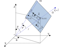Figure 1. Geometric configuration and coordinate parameters: a point M situated in the plane Σ_⊥ perpendicular and crossing Ω at point S. The point M is located in the vicinity of ray Ω and it ray-centered coordinates are q₁, q₂, and s. The center point O is at s=s₀.

Figure 1 presents the ray-centered coordinate system (s, q₁, q₂) used to formulate the equation (1) of the Gaussian beam amplitude u(s, q₁, q₂, t). This coordinate system is connected to any selected ray Ω. As a function of the local coordinates and at the receiver point, the solution of the Helmholtz equation as a solitary Gaussian beam is given by (1) [8].

In (1) t(s) is the travel time from the source along the selected ray, v is the propagation velocity, q^T represents the transpose of the vector, the quantities Q and P are 2 x 2 matrix called “dynamic quantities” satisfying the system ODE (2) in variations, called “dynamic ray tracing equations” (DRT) [11], [15].In a homogeneous medium with wave speed equal to the celerity c, the DRT equations can be written as:

The system of differential equations (2), is solved by introducing initial conditions specified at an arbitrary point (s = s₀) on the central ray. The initial conditions are also related to three other conditions along the whole rays [12]. These conditions are:

• Even though P and Q are not symmetrical the (P×Q^-1) must be symmetric matrix;
• Im(P×Q^-1) is a positive-definite matrix;
• (det[Q]≠ 0);

To find the initial values for Q and P, we use Hill’s [13] initial data for the Green’s function.

In (3), w₀ is the initial half beam width at the frequency f = w_r/2p, I is the identity matrix (2×2). Using the initial conditions in (3), we can find the general solution of (2), and can be written as follows:

In the case of homogeneous media, by using (4) in (1), we return to the representation of the amplitude u of the Gaussian beam in 3D:

Using the geometrical configuration illustrated in Figure 1, and introducing the spherical coordination system (r, q, φ), we can deduce the following factor (in 6) as a function of the distance (r) between the transmitter and the receiver:

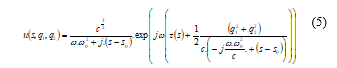
Finally, to calculate the full amplitude (u^GBS) at the receiver we must use an integral formulation as shown in (7). This integral will be calculated on all Gaussian beams described by their characteristic angle (d) from the source:

Where, Φφ is a quantity, generally complex-valued, which remains constant along the considered ray but may differ from ray to ray. It is called complex weight function. And the function u_φ(s, q₁, q₂) is the Gaussian beam connected with the ray.

In (7) the domain δ is centered on the central ray, it delimits the beams propagating in the vicinity of the central ray, chosen in such way that the Gaussian beam u_φ(s,q₁,q₂) outside this domain do not contribute effectively to the wave field. δ is a cone with a vertex angle φ.

For a homogeneous medium, on an observation point (M) the ray asymptotic solution of the Helmholtz equation is given by the following equation:

The GBS integral, in (7), may be evaluated asymptotically using the saddle-point method. Thus, this result must coincide with the above ray asymptotic solution in the regular region [12], [17]. Matching both asymptotic solution of (7) and (9) we can determine the complex weight function Φφ. Integral (7) is evaluated by numerical quadrature with regular increment Δφ. The equation (10) is used for the numerical computation.

After the formulation of the scattered filed using GBS method ((7) and (10)), we will analyze the influence of the main parameters of the Gaussian beam on the variation on the field amplitude. Then, we will compare the solution based on Gaussian beam with the analytical solution given by (9).

2.2.  Analysis of GBS method

Figure 2 compares the amplitude of field calculated by GBS method and ray asymptotic solution of the Helmholtz equation. This simulation (Figure 2) has been realized as a function of the distance (r in km) from the source to the receiver. The frequency equal to 10GHz, the beam width (ω₀) equal to 18λ (where λ is the wavelength) and the values of beams number (N) are : {133, 200, 400 and 600}. Magenta, red, green, blue and lines correspond to the GBS solution for different beams number, respectively 133, 200, 400 and 600 over which the summation is down. The black line represents the ray asymptotic solution. We can observe, that the beam density in the vicinity of the central ray offers satisfactory accuracy. In fact, when the number of the beams is more than 200, the GBS and the ray asymptotic are in good agreement. So, as with the usual techniques of ray tracing, a high beam density (200 for this case) is necessary for high accuracy.

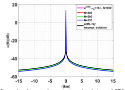Figure 2. Comparison between the ray asymptotic solution and GBS method for beam number N={133, 200, 400, 600} and beam width is 18λ.

In Figure 3, we compare the percentage error between the ray asymptotic solution and the GBS method. We can see even at a distance of 15 km the percentage error between the ray asymptotic solution and the GBS technique is lower than 10% for a beam density N = 200 and remains below 4% fo N = 400. In addition, one should note that the computations by GBS method exhibit no singularities when passing by the source point (r=0), unlike the ray asymptotic solution. This result confirms that by using the GBS method we can overcome some limitation of the ray asymptotic models. The proof of this result relies on the theory of systems of linear first order differential equations [14-16].

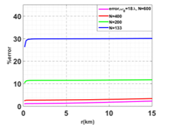Figure 3. Percentage error between the ray asymptotic solution and the GBS approximation of the Helmholtz’s wave equation for different beam number values.

Figure 4 illustrates the field amplitude calculated by GBS method (where N = 600 beams) and ray asymptotic solution. The different color lines correspond to the GBS solution for different beam width, {5λ, 8λ, 12λ, 15λ and 18λ}. This comparison shows that the GBS is ω₀ dependent. This beam initial parameter must be chosen optimally to guarantee sufficient accuracy.

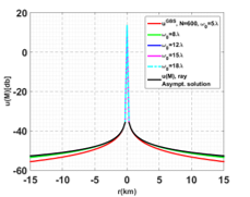Figure 4. Comparison between the ray asymptotic solution and GBS method for different beam width values: ω₀={5, 8, 12, 15, 18} and beam number equal to 600.

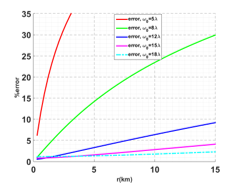Figure 5. Percentage error between the ray asymptotic solution and the GBS approximation of the Helmholtz’s wave equation for different beam width values.

To study in greater details the effect of the ω₀ parameters on the scattered field variation, we have simulated in Figure 5 the relative error between GBS solution and ray asymptotic solution. The relative error is normalized by ray asymptotic solution. The numerical analysis in Figure 5 indicates that for ω₀ = 18λ the relative error remains below 3% even at a distance 15 km  (and less than 2% at 5 km) from the source and the GBS solution match the ray asymptotic solution.

In the present paper, the GBS method was compared with another Gaussian approach called Gaussian Beam Launching (GBL). The formulations of GBL method are presented in the following part.

2.3.  Formulation of GBL method

The Gaussian Beam Launching (GBL) technique has been introduced and applied in the research published by H. T. Chou et al [17]. Consider a target (plate, disc, cylinder,…) illuminated by a Gaussian beam, the GBL method is applied to calculate the radiation integral of the target scattered fields. For the considered Gaussian beam, the incident magnetic field is given by the following form [4], [17]:

In (11), the distance between a point on the illuminated surface and the waist the incident Gaussian beam is denoted by r_i, the position vector in the Gaussian beam is defined by and b_i =k.w₀²/2, where k, w₀ are the wave number and the half beam-width respectively.

The electric fields scattered from the target surface (Σ) illuminated by the incident field is given by the integration of the incident Gaussian beam on the reflector surface (PO integral). This integral is written by (11):

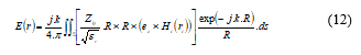Finally, by using (11) in (12) and solving the integral, we can compute the scattered field applying GBL formulation as in [4], [17].

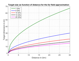Figure 6. Target size as a function of distance for far-field approximation: The Fraunhofer criterion of far-field.

In both GBS and GBL methods, it’s required to take into account the far-field approximation parameters (distance r, target size D, and wavelength l). In order that the phases and amplitudes of the waves arriving from different regions of the target do not vary considerably with the distance (r), the far-field region must be far enough away from the source. This region of the far field starts at a distance “r” given by the following equation (Fraunhofer criterion) [19]: r ≥ ((2.D²)/l).

Figure 6 shows the minimum far-field range as a function of the target dimensions D, and for different frequencies values. In this work, the simulations and measurements are realized for two frequency bands (5GHz and 10GHz).

3. Numerical and Experimental Results

3.1.  Experimental setup

The experimental measurements of RCS have been carried out on an anechoic chamber (8m x 5m x 5m) at Lab-STICC ENSTA Bretagne (see Figure 7).  The characteristics of various components of measurements system are:

• All walls are covered with absorbent material;
• The transmitter and receiver antennas are identical and there polarization is horizontal or vertical. They are placed on an angular rail that allows changing their position;
• A computer controls the Vectorial Network Analyzer (Anritsu 37347D) which operates in the frequency range from 40MHz to 20GHz and the positioning system;
• The NEWPORT positioning system with an angular resolution equal to 0.01° and an angle vary between -90° and 90°. An elevation motor for adjusting the height of the target;

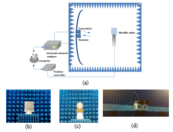Figure 7. (a) General description of the experimental setup, (b) Target plate, (c) Radar sphere calibration, (d) Transmitter and receiver antennas.

3.2.  Numerical simulation and experimental measurement of RCS

In the simulations illustrated in Figure 8, we set the azimuth angles φ_i to zero; the incident angle θ_i varies from −10˚ to 10˚ and the other acquisition parameters are: f = 10GHz, the beam width ω₀ = 2λ, beams number N = 200. The GBS is compared with the Gaussian GBL method, the asymptotic PO model, and the rigorous MoM method (in FEKO). Comparing the curve of RCS using GBS is in the blue line, GBL technique in red line with the other models; we observe that they match rigorously the PO solution and MoM for the main beam. In fact, GBS and GBL accurately model the main beam, without mitigation, the diagrams are also consistent, and the modeled peak width and location match the PO and MoM solutions.

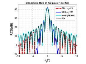Figure 8. Monostatic RCS of a PEC flat plate computed using GBS, GBL techniques, for beam width ω₀ = 2λ and compared with PO and MoM methods: f =10GHz, vv

From Figure 8 we can conclude that the GBS method models very well the variation of the scattered field in the specular direction. However, we observe that the GBL method simulates the secondary lobes better than the GBS method. The deviation between the curves in outside specular direction can be considered through broadening the range of validity of the GBS by taking into account the edge diffraction. To consider the edge diffraction contribution, we need to use the method of the Geometric Theory of Diffraction (GTD) [18]. In fact, the diffracted field when incident field strikes the edges is calculated from the GTD and is accounted in the complex weight function in the integral (7).

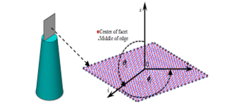Figure 9. Geometry of a flat plate (30 cm ×30 cm) meshed with triangular patches.

Figure 9 represents the geometry of a flat plate meshed with a triangular patch (using CATIA software). In this geometric configuration, each facet is represented by a triangle node (in blue) with a central point in red color (bright points) and black cross in the middle of the external edge. This geometric configuration and this mesh will be used in the calculation of RCS by the two techniques GBL and GBS + GTD.

The simulated (using GBS, GBL, PO, and MoM) and measured RCS results of PEC plate are shown in Figure 10 and Figure 11. The acquisition parameters are: frequency of 10GHz, the incident angle θ_i varies from −60˚ to 60˚, the azimuthal scattering angle equal to 0°, the size of a flat plate as function of the wavelength is (10λ x10λ), the beam width of w₀ =2l, beam number density equal to 200 and the polarizations are hh and vv in Figure 10 and Figure 11 respectively.

The comparison between GBS, with accounting and without accounting the edge diffraction contribution, is illustrated in Figure 10. The evaluation GBS technique is also performed with GBL, PO, and MoM methods. From this comparison results, we can see that when the diffraction is accounted we obtain values of the RCS which get closer to those given by the experimental measurements and the rigorous MoM method. In addition, where the polarization state is hh and vv respectively, we remark that the PO model is insufficient in computing of edge plate diffraction contributions, although the agreement of GBS+GTD and GBL with the rigorous MoM solution and measured data are good in the most of scattering angles (particularly in vv polarization).

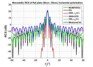Figure 10. Comparison between GBS, GBS+GTD, GBL, the numerical models and the experimental measurements in hh polarization: (30cm × 30cm).

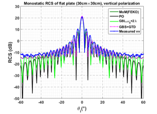Figure 11. Comparison between GBS+GTD, GBL, the numerical models and the experimental measurements in vv polarization: (30cm ×30cm).

The experimental validation results show that GBS method gives a higher accurate representation of the scattered field and offer very interesting perspectives for complex targets such as cavity and corner for example. Figure 12 shows the evolution of the RCS of a metallic dihedral corner reflector realized using Ray Launching-Geometrical Optics (RL-GO) and MoM methods and also experimental measurement at a frequency of 5GHz.

In Figure 12, we can see that the curve of measured RCS is near to that simulated by MoM method. These results will serve as a basis for evaluating the development of the GBS method in our future work.

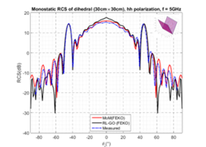Figure 12. RCS of rectangular dihedral corner reflector (f = 5GHz): Experimental and numerical models.

4. Conclusion and future work

In this study, the RCS of radar targets has been investigated by using a new technique called Gaussian Beam Summation (GBS). In the GBS technique, the total field at the receiver is represented by the integral over all Gaussian beams propagating in the vicinity of the receiver. To study the performance of the chosen GBS method, we have carried out it theoretical formulation and we have study the influence main Gaussian parameters (beams width, the density of beams number) on the field amplitude. Then, we have introduced a numerical simulation of the RCS of a PEC plate using GBS method. The results obtained using GBS were compared with those simulated trough GBL, PO and MoM methods. In addition, we have presented the experimental measurements of RCS of canonical and complex targets. The results of RCS using GBS method were compared and validated by the experimental measurements.

The study of the RCS of different complex objects (including dihedral and trihedral corner reflector) using GBS method is one of the perspectives of the work presented in this paper.

Conflict of Interest

The authors declare no conflict of interest.

Acknowledgment

We would like to thank the DGA (Direction Générale de l’Armement, France)-MRIS for their support of the SOFAGEMM project, where this work is in progress. Acknowledgments are also addressed to Mr. Hervé TRÉBAOL (Specialized Instructor Mechanical Design in ENSTA Bretagne) for these collaborations with us.

1. F.Weinmann, “Ray tracing with PO/PTD for RCS modeling of large complex objects,” IEEE Trans. Antennas and Propagation., 54( 6), 1797–1806, Jun. 2006. DOI: 10.1109/TAP.2006.875910
2. R. Harrington, “Field computation by moment methods,” Wiley-IEEE Press, 1993.
3. H. T. Chou and P. H. Pathak, “Uniform asymptotic solution for electromagnetic reflection and diffraction of an arbitrary Gaussian beam by a smooth surface with an edge,” Radio. Science., 32(14), 1319-1336, 1997. DOI: 10.1029/97RS00713
4. P.O. Leye, A. Khenchaf, and P. Pouliguen, “The Gaussian Beam Summation and the Gaussian Launching Methods in Scattering Problem,” J. Elect. Analysis and Applications., 8, 219-225, 2016. DOI: 10.4236/jemaa.2016.810020
5. H. Ghanmi, A. Khenchaf, P. Pouliguen and P. O. Leye, “Study of RCS of complex target: Experimental measurements and Gaussian beam summation method,” IEEE Conference on Antenna Measurements & Applications (CAMA), Tsukuba, pp. 196-199, 2017. DOI: 10.1109/CAMA.2017.8273399
6. M. Katsav and E. Heyman, “Gaussian Beam Summation Representation of Beam Diffraction by an Impedance Wedge: A 3D Electromagnetic Formulation Within the Physical Optics Approximation,” IEEE Trans. Antennas Propagation., 60(12), pp. 5843-5858, 2012. DOI: 10.1109/TAP.2012.2207694
7. V. Červený, “Summation of paraxial Gaussian beams and of paraxial ray approximations in inhomogeneous anisotropic layered structures,” Seismic waves. Complex 3-D Structures., 10, 121–159, 2000. https://doi.org/10.1111/j.1365-246X.2009.04442.x
8. M. M. Popov, “A new method of computation of wave fields using Gaussian beams,” Wave Motion., 4, 85-97, 1982. https://doi.org/10.1016/0165-2125(82)90016-6
9. V. Červený, “Expansion of a Plane Wave into Gaussian Beams,” Stidia geoph. And geod., 26, 120 – 131, 1982. DOI: 10.1007/BF01582305
10. V. Červený,“Seismic Ray Theory,” Cambridge: Cambridge University Press, 2001.
11. M. M. Popov, “New method of computation of wave fields in high-frequency approximation,” J. Soviet Math., 20(1) ,1869–1882, 1982. https://doi.org/10.1007/BF01119372
12. V. Červený,, “Gaussian beam synthetic seismograms,” Journal. Geoph., 58, 44-72, 1985.
13. N. R. Hill, “Gaussian beam migration,” Geophysics, 55(11), 1416-1428, 1990. https://doi.org/10.1190/1.1442788
14. V. Červený,Červený, «Computation of wave field in homogeneous media,» Geophys. J. R. astr. Soc., 70, 109-128, 1982. DOI: 10.1111/j.1365-246X.1982.tb06394.x
15. B. S. White, A. Norris, A. Bayliss and R. Burridge, “Some remarks on the Gaussian beam summation method,” Geoph. J. Royal. Astro. Society., 89, 579-636 , 1987. https://doi.org/10.1111/j.1365-246X.1987.tb05184.x
16. B. Bleistein, “Mathematics of Modeling, Migration and Inversion with Gaussian Beams,” Colorado, USA, 2008. DOI: 10.3997/2214-4609.201405084
17. H. T. Chou, P. Pathak and R. J. Burkholder, “Novel Gaussian Beam Method for the Rapid Analysis of Large Reflector Antennas,” IEEE Trans. Antennas. Propagation., 49(16), 880-893, 2001. DOI: 10.1109/8.931145
18. J. B. Keller, “Geometrical Theory of Diffraction,” J.Optical Society of America, 52, 116 – 130, 1962. https://doi.org/10.1364/JOSA.52.000116
19. Warren L. Stutzman, Gary A. Thiele. “Antenna Theory and Design”. John Wileys & Sons, Inc., 1997.

(Click Here)

(Click Here)