1. Introduction

Sequence alignment is a fundamental and well-studied problem in the biological sciences. In this problem, we are given two sequences _A[1 : _m] = _aa₂···_am and B[1 : _n] = _b1b₂···_bn and we are required to find the score of the best alignment and possibly also an alignment with this best score. When aligning two sequences, we may insert gaps into the sequences. The score of an alignment is determined using a matching (or scoring) matrix that assigns a score to each pair of characters from the alphabet in use as well as a gap penalty model that determines the penalty associated with a gap sequence. In the linear gap penalty model, the penalty for a gap sequence of length _{k >} 0 is _kg, where _g is some constant while in the affine model this penalty is g_open + (k − 1) ∗ g_ext. The affine model more accurately reflects the fact that opening a gap is more expensive than extending one. Two versions of sequence alignment–global and local–are of interest. In global alignment, the entire _A sequence is to be aligned with alignment score. The alphabet for DNA, RNA, and protein sequences is, respectively, {A, T, G, C}, {A, U, G, C}, and {A, C, D, E, F, G, H, I, K, L, M, N, P, Q, R, S, T, V, W, Y}.

Figure 1 illustrates these concepts using the DNA sequences _A[1 : 8] = {AGTACGCA} and _B[1 : 5] = {TATGC}. The symbol ‘_’ denotes the gap character. The alignment of Figure 1(a) is a global alignment and that of Figure 1(b) is a local one. To score the alignments, we have used the linear penalty model with g = ₋2 and the scores for pairs of aligned characters, which are taken from BLOSUM62 matrix in [1], are c(T,T) = 5, c(A,A) = 4, c(C,C) = 9, c(G,G) = 6, and c(_C,T) = ₋1. The score for the shown global alignment is 17 while that for the shown local alignment is 23. If we were using an affine penalty model with _gopen = −4 and _gext = ₋2, then the penalty for each of the gaps in positions 1 and 8 of the global alignment would be ₋4 and the overall score for the global alignment would be 13.

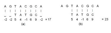Figure 1: Example alignments using the linear gap penalty model. (a) Global alignment (b) Local alignment

In [2], the authors first proposed an _O(_mn) time algorithm, called Needleman-Wunsch(NW) algorithm, for global alignment using the linear gap model. This algorithm requires _O(_n) space when only the score of the best alignment is to be determined and _O(_mn) space when the best alignment is also to be determined. In [3], the authors proposed a new algorithm called SmithWaterman(SW) algorithm, which modified the NW algorithm so as to determine the best local alignment. In [4], the author proposed a dynamic programming algorithm called Gotoh algorithm, for sequence alignment using an affine gap penalty model. The asymptotic complexity of the SW and Gotoh algorithms is the same as that of the NW algorithm.

When _mn is large and the best alignment is sought, the space, _O(_mn), required by the algorithms of NW, SW and Gotoh exceeds what is available on most computers. The best alignment for these large instances can be found in [5] using sequence alignment algorithms derived from Hirschberg’s linear space divide-and-conquer algorithm for the longest common subsequence problem. In [6], the authors developed a Myers-Miller alignment algorithm. It is the linear space _O(_mn) time version of Hirschberg’s algorithm for global sequence alignment using an affine gap penalty model. And in [7], the authors do this for local alignment.

In an effort to speed sequence alignment, fast sequence-alignment heuristics have been developed. As in [8, 9, 10],BLAST, FASTA, and Sim2 are a few examples of software systems that employ sequence alignment heuristics. Another direction of research, also aimed at speeding sequence alignment, has been the development of parallel algorithms. Parallel algorithms for sequence alignment may be found in [11]-[19], for example.

In this paper, we focus on reducing the number of cache misses that occur in the computation of the score of the best alignment as well as in determining the best alignment. Although we explicitly consider only the linear gap penalty model, our methods readily extend to the affine gap penalty model. Our interest in cache misses stems from two observations–(1) the time required to service a last-level-cache (LLC) miss is typically 2 to 3 orders of magnitude more than the time for an arithmetic operation and (2) the energy required to fetch data from main memory is typically between 60 to 600 times that needed when the data is on the chip. As a result of observation (1), cache misses dominate the overall running time of applications for which the hardware/software cache prefetch modules on the target computer are ineffective in predicting future cache misses. The effectiveness of hardware/software cache prefetch mechanisms varies with application, computer, and compiler. So, if we are writing code that is to be used on a variety of computer platforms, it is desirable to write cache-efficient code rather than to rely exclusively on the cache prefetching of the target platform. Even when the hardware/software prefetch mechanism of the target platform is very effective in hiding memory latency, observation (2) implies excessive energy use when there are many cache misses.

This paper is an extension of work originally in [20], which has been presented by us in the 2015 IEEE 5th international conference on Computational Advances

in Bio and Medical Sciences (ICCABS). The main contributions are

1. cache efficient single-core and multi-core algorithms to determine the score of the best alignment;
2. cache efficient single-core and multi-core algorithms to determine the best alignment.

The rest of the paper is organized in the following way. In Section 2, we describe our cache model. Our cache-efficient algorithms for scoring and alignment are developed and analyzed in Section 3. Experimental results are presented in Section 4. In Section 5, we present a discussion of these results and in Section 6, we present the limitations of our work. Finally, we conclude in Section 7.

2. Cache Model

For simplicity in the analysis, we assume a single cache comprised of _s lines of size _w words (a word is large enough to hold a piece of data, typically 4 bytes) each. So, the total cache capacity is _sw words. The main memory is partitioned into blocks also of size _w words each. When the program needs to read a word that is not in the cache, a cache miss occurs. To service this cache miss, the block of main memory that includes the needed word is fetched and stored in a cache line, which is selected using the LRU (least recently used) rule. Until this block of main memory is evicted from this cache line, its words may be read without additional cache misses. We assume the cache is written back with write allocate. Write allocate means that when the program needs to write a word of data, a write miss occurs if the block corresponding to the main memory is not currently in cache. To service the write miss, the corresponding block of main memory is fetched and stored in a cache line. Write back means that the word is written to the appropriate cache line only. A cache line with changed content is written back to the main memory when it is about to be overwritten by a new block from main memory.

Rather than directly assess the number of read and write misses incurred by an algorithm, we shall count the number of read and write accesses to main memory.

Every read and write miss makes a read access. A read and write miss also makes a write access when the data in the replacement cache line is written to main memory.

We emphasize that the described cache model is a very simplified model. In practice, modern computers commonly have two or three levels of cache and employ sophisticated adaptive cache replacement strategies rather than the LRU strategy described above. Further, hardware and software cache prefetch mechanisms are often deployed to hide the latency involved in servicing a cache miss. These mechanisms may, for example, attempt to learn the memory access pattern of the current application and then predict the future need for blocks of main memory. The predicted blocks are brought into cache before the program actually tries to read/write from/into those blocks thereby avoiding (or reducing) the delay involved in servicing a cache miss. Actual performance is also influenced by the compiler used and the compiler options in effect at the time of compilation. As a result, actual performance may bear little relationship to the analytical results obtained for our simple cache model. Despite this, we believe the simple cache model serves a useful purpose in directing the quest for cache-efficient algorithms that eventually need to be validated experimentally.

3. Cache Efficient Algorithms

3.1. Scoring Algorithms

3.1.1     Needleman-Wunsch and Smith-Waterman algorithm

Let _Hij be the score of the best global alignment for

A[1 : _i] and _B[1 : _j]. We wish to determine _Hmn. In [2], the authors derived the following dynamic programming equations for _H using the linear gap penalty model. These equations may be used to compute _Hmn.

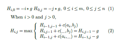 Hi−1,j +c(ai,_) = Hi−1,j −g where _c(_ai,b_j) is the match score between characters _ai and _bj and _g is the gap penalty.

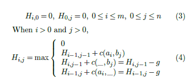
For local alignment, _Hij denotes the score of the best local alignment for _A[1 : _i] and _B[1 : _j]. In [3], the Smith-Waterman equations for local alignment using the linear gap penalty model are:

Several authors (in [5, 6], for example) have observed that the score of the best local alignment may be determined using a single array _H[0 : _n] as in algorithm Score(Algorithm 1.)

Algorithm 1 Smith-Waterman scoring algorithm

1: Score(A[1 : m],B[1 : n]) 2: for j ← 0 to n do

3:             _H[_j] ← 0 //Initialize row 0

4: end for 5: for i ← 1 to m do

6:            _diag ← 0 // Compute row i

7:            for j ← 1 to n do

8:                nextdiag ← H[j]

9:           H[j] ← max{0,diag + c(A[i],B[j]),H[j − 1] − g,H[j]−g}

10:             diag ← nextdiag

11:        end for

12: end for

13: return H[n]

The scoring algorithm for the Needleman and Wunsch algorithm is similar. It is easy to see that the time complexity of the algorithm of Algorithm 1 is _O(_mn) and its space complexity is _O(_n).

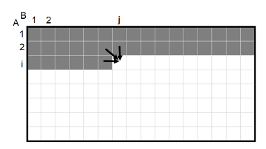Figure 2: Memory access pattern for Score algorithm(Algorithm 1).

For the (data) cache miss analysis, we focus on read and write misses of the array _H and ignore misses due to the reads of the sequences _A and _B as well as of the scoring matrix _c (notice that there are no write misses for _A, _B, and _c). Figure 2 shows the memory access pattern for _H by algorithm _Score. The first row denotes the initialization of _H and subsequent rows denote access for different value of _i (i.e., different iterations of the _{for i} loop). The computation of _Hij is done using a single one-dimensional array _H[], following the _i’th iteration of the _{for i} loop, _H[_j] = _Hij. In each iteration of this loop, the elements of _H[] are accessed left-to-right. During the initialization loop, _H is brought into the cache in blocks of size _w. Assume that _n is sufficiently large so that _H[] does not entirely fit into the cache. Hence, at some value of _j, the cache capacity is reached and further progress of the initialization loop causes the least recently used blocks of _H[]

(i.e., blocks from left to right) to be evicted from the cache. The evicted blocks are written to main memory as they have been updated. So, the initialization loop results in _n/w read accesses and (approximately) _n/w write accesses (the number of write accesses is actually n/w −_s). Since the left part of _H[] has been evicted from the cache by the time we start the computation for row _i (_{i >} 0), each iteration of the _{for i} loop also results in _n/w read accesses and approximately _n/w write accesses. So, the total number of read accesses is (_m+1)_n/w ≈ _mn/w and the number of write accesses is also _{≈ mn/w}. The number of read and write accesses is ≈ 2mn/w, when n is large.

We note, however, that when _n is sufficiently small that _H[] fits into the cache, the number of read accesses is _n/w (all occur in the initialization loop) and there are no write accesses. In practice, especially in the case of local alignment involving a very long sequence, one of the two sequences _A and _B is small enough to fit in the cache while the other may not fit in the cache. So, in these cases, it is desirable to ensure that _A is the longer sequence and _B is the shorter one so that _H fits in the cache entirely. This is accomplished by swap A and B sequences.

When _{m < n} and _H[1 : _m] fits into the cache and

H[1 : n] does not, algorithm Score incurs O(mn/w) read/write accesses, while swap A and B incurs _O(_m/w) read/write accesses.

3.1.2. Diagonal Algorithm

An alternative to computing the score by rows is to compute by diagonals. While this uses two one-dimensional arrays rather than one, it is more readily parallelized than _Score as all elements on a diagonal can be computed at the same time; elements on a row need to be computed in sequence. Algorithm 2 Diagonal scoring algorithm

1: Diagonal(A[1 : m],B[1 : n])

2: d2[0] ← d1[0] ← d1[1] ← 0

3: for d ← 2 to m+n do

4: x ← (d <= m?0 : d−m);y ← (d <= n?d : n); for i ← x to y do

j ← d−i

diag ← next+c(A[i]+B[j]) left ← d1[i−1]−g up ← d1[i]−g next ← d2[i]

11:                d2[i] ← max{0,diag,left,up}

12:        end for

13:         swap(d1,d2)

14: end for

15: return d1[n]

Algorithm _Diagonal (Algorithm 2) uses two onedimensional arrays _d1[] and _d2[], where _d2[] stores the scores for the (_d−2)th diagonal data and _d1[] stores them for the (_d−1)th diagonal. When we compute the element _Hi,j in the _dth diagonal, the previous diagonal element _Hi−1,j−1 is fetched from _d2[] and the previous left element H_i−1,j and previous upper element H_i,j−1 are fetched from _d1[]. The calculated _Hi,j overwrites the old value in _d2[].

The total number of read accesses is _mn/w for each diagonal array and the total number of write accesses is mn/w for both arrays combined. The number of cache misses for Diagonal is approximately 3mn/w when n is large.

3.1.3. Strip Algorithm

When neither _H[1 : _m] nor _H[1 : _n] fits into the cache, accesses to main memory may be reduced by computing _Hij by strips of width _q such that _q consecutive elements of _H[] fit into the cache. Specifically, we partition _H[1 : _n] into _n/q strips of size _q (except possibly the last strip whose size may be smaller than _q) as in Figure 3. First, all _Hij in strip 0 are computed, then those in strip 1, and so on. When computing the values in a strip, we need those in the rightmost column of the preceding strip. So, we save these rightmost values in a one-dimensional array _strip[0 : _m]. The algorithm is given in Algorithm 3. We note that sequence alignment by strips has been considered before. For example, in [12], the authors using the similar approach in their GPU algorithm. Their use differs from ours in that they compute the strips in pipeline fashion with each strip assigned to a different pipeline stage in round robin fashion and within a strip, the computation is done by anti-diagonals in parallel. On the other hand, we do not pipeline the computation among strips and within a strip, our computation is by rows. Algorithm 3 Strip scoring algorithm

1: Strip(A[1 : m],B[1 : n])

2: for j ← 1 to m do

3:            strip[j] ← 0 //leftmost strip

4: end for

5: for t ← 1 to n/q do 6:    for j ← t∗q to t∗q +q −1 do

7:                 _H[_j] ← 0 //Initialize first row

8:       end for for i ← 1 to m do

diag ← strip[i−1]

H[t∗q −1] ← strip[i]

for j ← t∗q to t∗q +q −1 do nextdiag ← H[j]

H[j] ← max{0,diag+c(A[i],B[j]),H[j−1]− g,H[j]−g}

15:                  diag ← nextdiag

16:            end for

17:                strip[i] ← H[t∗q +q −1]

18:        end for

19: end for

20: return H[n]

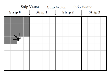Figure 3: Memory access pattern for Strip algorithm (Algorithm 3).

It is easy to see that the time complexity of algorithm _Strip is _O(_mn) and that its space complexity is O(_m+_n). For the cache misses, we focus on those resulting from the reads and writes of _H[] and _strip[]. The initialization of _strip results in _m/w read accesses and approximately the same number of write accesses. The computation of each strip makes the following accesses to main memory:

1. _q/w read accesses for the appropriate set of _q entries of _H for the current strip and _q/w write accesses for the cache lines whose data are replaced by these _H The write accesses are, however, not made for the first strip.
2. _m/w read accesses for _strip and _m/w write accesses. The number of write accesses is less by _s for the last strip.

So, the overall number of read accesses is _m/w +

(q/w +m/w)∗n/q = m/w +n/w +mn/(wq) and the number of write accesses is approximately the same as this. So, the total number of main memory accesses is ≈ 2mn/(wq) when m and n are large.

3.2. Alignment Algorithms

In this section, we examine algorithms that compute the alignment that results in the best score rather than just the best score. While in the previous section we explicitly considered local alignment and remarked that the results readily extend to global alignment, in this section we explicitly consider global alignment and remark that the methods extend to local alignment.

3.2.1. Myers and Miller’s Algorithm

When aligning very long sequences, the _O(_mn) space requirement of the full-matrix algorithm exceeds the available memory on most computers. For these instances, we need a more memory-efficient alignment algorithm. In [6], Myers and Miller have adapted Hirschberg’s linear space algorithm for the longest common subsequence problem to find the best global alignment in linear space. Its time complexity is _O(_mn). However, this linear space adaptation performs about twice as many operations as does the full-matrix algorithm. In [11], the authors have developed a hybrid algorithm, FastLSA, whose memory requirement adapts to the amount of memory available on the target computing platform. In this section and the next, we focus on the adaptation of Myers-Miller algorithm.

It is easy to see that an optimal (global) alignment is comprised of an optimal alignment of _A[1 : _m/2] and B[1 : _j] and an optimal alignment of _A[_m : _m/2 + 1] (_A[_m : _i] is the reverse of _A[_i : _m]) and _B[_n : _j +1] for some _j, 1 ≤ _j ≤ _n. The value of _j for which this is true is called the optimal crossover point. Myers and Miller’s linear space algorithm for alignment determines the optimal alignment by first determining the optimal crossover point (_si,sj) where _si = _m/2, and then recursively aligning _A[1 : _m/2] and _B[1 : _sj] as well as A[_m : _m/2+1] and _B[_n : _sj +1]. Equivalently, an optimal alignment of _A[1 : _m] and _B[1 : _n] is an optimal alignment of _A[1 : _m/2] and _B[1 : _sj] concatenated with the reverse of an optimal alignment of _A[_m : _m/2+1] and _B[_n : _sj +1]. Hence, an optimal alignment is comprised of a sequence of optimal crossover points. This is depicted visually in Figure 4. Figure 4(a) shows alignments using 3 possible crossover points at row _m/2 of H. Figure 4(b) shows the partitioning of the alignment problem into 2 smaller alignment problems (shaded rectangles) using the optimal crossover point (meeting point of the 2 shaded rectangles) at row _m/2. Figure 4(c) shows the partitioning of each of the 2 subproblems of Figure 4(b) using the optimal crossover points for these subproblems (note that these crossovers take place at rows _m/4 and 3_m/4, respectively). Figure 4(d) shows the constructed optimal alignment, which is presently comprised of the 3 determined optimal crossover points.

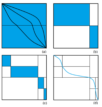Figure 4: An alignment as crossover points. (a) Three alignments (b) Optimal crossover for m/2 (c)Optimal crossover points at m/4 and 3m/4 (d) Best alignment Algorithm 4 Myers and Miller algorithm

1: MM(A[1 : m],B[1 : n],path[1 : m]) 2: if m <= 1 or n <= 1 then

3: Linear search to find optimal crossover point [si,sj]

4:            path[m] ← [si,sj]

5: else

6:             H_top ← MScore

7:             H_bot ← MScore

8: Linear search to find optimal crossover point [si,sj]

9:            MM,path

10:        path

11:         MM                                                      ,path

12: end if

The Myers and Miller algorithm, _MM (Algorithm 4), uses a modified version of the linear space scoring algorithm _Score (Algorithm 1) to obtain the scores for the best alignments of _A[1 : _i] and _B[1 : _j], 1 ≤ _i ≤ _m/2, 1 ≤ _j ≤ _n as well as for the best alignments of A[m : i] and B[m : j], m/2 < i ≤ m, 1 ≤ j ≤ n. This modified version _MScore differs from _Score only in that _MScore returns the entire array _H rather than just _H[_n]. Using the returned _H arrays for the forward and reverse alignments, the optimal crossover point for the best alignment is computed as in algorithm _MM (Algorithm 4). Once the optimal crossover point is known, two recursive calls are made to optimally align the top and bottom halves of _A with left and right parts of _B. The approximately time complexity for iteration k is _O(2_mn/2^k), hence the total time complexity is rough 2_mn.

In each level of recursion, the number of main memory accesses is dominated by those made in the calls to MScore. From the analysis for _Score, it follows that when _n is large, the number of accesses to main memory is ≈ 2mn/w(1+1/2+1/4+···) ≈ 4mn/w.

3.2.2. Diagonal Myers and Miller Algorithm

Let Mdiagonal be algorithm Diagonal (Algorithm 2) modified to return the entire _H array rather than just _H[_n]. Our diagonal Myers and Miller algorithm (_MMDiagonal) replaces the two statements in algorithm _MM (Algorithm 4) that invoke _MScore with a test that causes _Mdiagonal to be used in place of MScore when both of _m and _n are sufficiently long.

From the analysis for _Diagonal, it follows that when m and _n are large, the number of accesses to main memory is ≈ 3mn/w(1+1/2+1/4+···) ≈ 6mn/w.

3.2.3. Striped Myers and Miller Algorithm

Let _MStrip be algorithm _Strip (Algorithm 3) modified to return the entire _H array rather than just _H[_n]. Our striped Myers and Miller algorithm (_MMStrip) replaces the two statements in algorithm _MM (Algorithm 4) that invoke _MScore with a test that causes MStrip to be used in place of _MScore when both of m and _n are sufficiently long.

From the analysis for _Strip, it follows that when _m and _n are large, the number of accesses to main memory is ≈ 2mn/(wq)(1+1/2+1/4+···) ≈ 4mn/(wq).

3.3. Parallel Scoring Algorithms

3.3.1. Parallel Score Algorithm

As remarked earlier in _Score algorithm, the elements in a row of the score matrix need to be computed sequentially from left to right because of data dependencies. So, we are unable to parallelize the inner _for loop of _Score (Algorithm 1). Instead, we adopt the unusual approach of parallelizing the outer _for loop while computing the inner loop sequentially using a single processor. Initially, processor _s is assigned to do the outer loop computation for _i = _s, 1 ≤ _i ≤ _p, where _p is the number of processors. Processor _s begins after a suitable time lag relative to the start of processor _s−1 so that the data it needs for its computation has already been computed by processor _s−1. That is, processor 1 begins the inner loop computation for _i = 1 at time 0, then, with a suitable time lag, processor 2 begins the outer loop computation for _i = 2, then, with a further lag, processor 3 begins the _i = 3 computation and so on. When a processor has finished with its iteration i computation, it starts on iteration _i+_p of the outer loop. Synchronization primitives are used to ensure suitable time lags. The time complexity of the resulting p-core algorithm PP_Score is O(mn/p).

3.3.2. Parallel Diagonal Algorithm

The inner _for loop of _Diagonal (Algorithm 2) is easily parallelized as the elements on a diagonal are independent and may be computed simultaneously. So, in our parallel version, we divide the diagonal _d into _p blocks, where _p is the number of processors. We assign a block to each processor from left to right as in Figure 5. The time complexity of the resulting _p-core algorithm PP_Diagonal is O(mn/p).

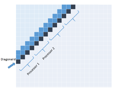Figure 5: Parallel Diagonal algorithm.

3.3.3. Parallel Strip Algorithm

In the _Strip scoring algorithm, we partition the score matrix _H into _n/q strips of size _q (Figure 3) and compute the strips one at a time from left to right. Inside a strip, scores are computed row by row from top to bottom. We see that the computation of one strip can begin once the first row of the previous strip has been computed. In our parallel version of this algorithm, processor _i is initially assigned to compute strip _i, 1 _{≤ i ≤ p}. When computing a value in its assigned strip, a processor needs to wait until the values (if any) needed from the strip to its left have been computed. When a processor completes the computation of strip _j, it proceeds with the computation of strip _j +_p. Figure 6 shows a possible state in the described parallel strip computation strategy. We maintain an array _signal[] such that _signal[_r] = _s+1 iff the row _r computation for strips 1 through _s has been completed. This array enables the processor working on the strip to its right to determine when it can begin the computation of its r’th row. The time complexity of the resulting parallel strip algorithm, PP_Strip, is O(mn/p).

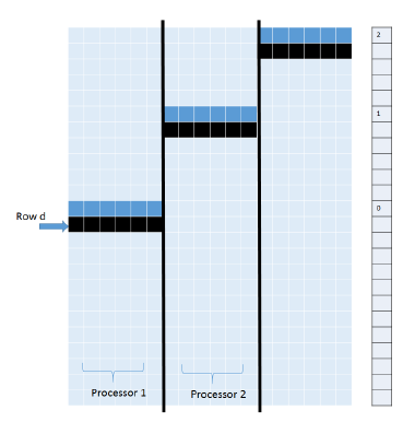Figure 6: Parallel Strip algorithm.

3.4. Parallel Alignment Algorithms

In the single-core implementation, we divide the _H matrix into two equal size parts and apply the scoring algorithm to each part. Then, we determine the optimal crossover point where the sum of the scores from both directions is maximum. This crossover point is used to divide the matrix into two smaller score matrices to which this decomposition strategy is recursively applied. The first application of this strategy yields two independent subproblems and following an application of the strategy to each of these subproblems, we have 4 even smaller subproblems. Following _k rounds, we have 2^k independent subproblems.

For the parallel version of alignment algorithms, we employ the following strategies:

• When the number of independent matrices is small, each matrix is computed using the parallel version of score algorithms _PP__Score, PP_Diagonal and PP_Strip; where p processors are assigned to the parallel computation. In other words, the matrices are computed in sequence.
• When the number of independent matrices is large, each matrix is computed using the single-core al-

gorithms Score, Diagonal and Strip. Now, p matrices are concurrently computed.

        Let           PP_MM,                PP_MMDiagonal             and

PP__MMStrip, respectively, denote the parallel versions of MM, MMDiagonal and MMStrip.

4. Results

4.1. Experimental Settings and Test Data

We implemented the single-core scoring and alignment algorithms in C and the multi-core scoring and alignment algorithms in C and OpenMP. The relative performance of these algorithms was measured on the following platforms:

1. Intel Xeon CPU E5-2603 v2 Quad-Core processor

1.8GHz with 10MB cache.

2. Intel I7-x980 Six-Core processor 3.33GHz with 12MB LLC cache.
3. Intel Xeon CPU E5-2695 v2 2xTwelve-Core processors 2.40GHz with 30MB cache.

For convenience, we will, at times, refer to these platforms as Xeon4, Xeon6, and Xeon24 (i.e., the number of cores is appended to the name Xeon).

All codes were compiled using the gcc compiler with the O2 option. On our Xeon4 platform, we used the “perf” [21] software to measure energy usage through the RAPL interface. So, for this platform, we report cache misses and energy consumption as well as running time. For the Xeon6 and Xeon24 platforms, we provide the running time only.

For test data, we used randomly generated protein sequences as well as real protein sequences obtained from the Globin Gene Server[22] and DNA/RNA/protein sequences from the National Center for Biotechnology Information (NCBI) database [23]. We used the BLOSUM62[1] scoring matrix for all our experiments. The results for our randomly generated protein sequences were comparable to those for similarly sized sequences used from the two databases [22] and [23]. So, we present only the results for the latter data sets here.

4.2. Xeon E5-2603 (Xeon4)

4.2.1. Score Algorithms

Figure 7 and Table 1 give the number of cache misses on our Xeon4 platform for different sequence sizes. The last two columns of Table 1 gives the percent reduction in the observed cache miss count of _Strip relative to Score and Diagonal. Strip has the fewest cache misses followed by Score and Diagonal (in this order). Strip reduces cache misses by up to 86_.2% relative to _Score and by up to 92_.3% relative to _Diagonal.

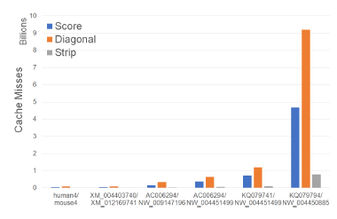Figure 7: Cache misses of scoring algorithms, in billions, on Xeon4.

Figure 8 and Table 2 give the running times of our scoring algorithms on our Xeon4 platform. In the figure, the time is in seconds while in the table, the time is given using the format _hh : _mm : _ss. The table also gives the percent reduction in running time achieved by Strip relative to Score and Diagonal.

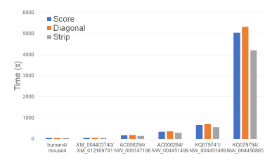Figure 8: Run time of scoring algorithms, in seconds, on Xeon4.

As can be seen, on our Xeon4 platform, _Strip is the fastest followed by _Score and _Diagonal (in this order). Strip reduces the running time by up to 17_.5% relative to _Score and by up to 22_.8% relative to _Diagonal. The reduction in running time, while significant, isn’t as much as the reduction in cache misses possibly due to the effect of cache prefetching, which reduces cache induced computational delays.

Figures 9 and Tables 3 give the CPU and cache energy consumed, in joules, by our Xeon4 platform.

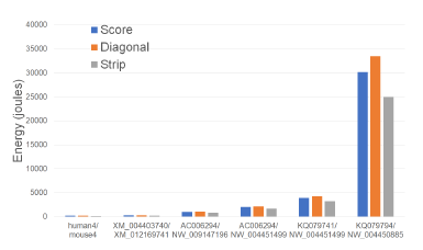Figure 9: CPU and cache energy consumption of scoring algorithms, in joules, on Xeon4.

On our datasets, _Strip required up to 18_.5% less CPU and cache energy than _Score and up to 25_.5% less than _Diagonal. It is interesting to note that the energy reduction is comparable to the reduction in running time suggesting a close relationship between running time and energy consumption for this application.

4.2.2. Parallel Scoring Algorithms

Figure 10 and Table 4 give the number of cache misses on our Xeon4 platform for our parallel scoring algorithms. _PP__Strip has the fewest cache misses followed by PP_Score and PP_Diagonal (in this order). _PP__Strip reduces cache misses by up to 98_.1% relative to _PP__Score and by up to 99_.1% relative to PP__Diagonal. We observe also that the total cache misses for _PP__Score is slightly higher than for _Score for smaller instances and lower for larger instances. PP__Diagonal, on the other hand, consistently has more cache misses than Diagonal. PP_Strip exhibits a significant reduction in cache misses. This is because we chose the strip width to be such that _p strip rows fit in this cache. Most of the cache misses in the _Strip are from the vector that transfers boundary results from one strip to the next. When _p strips are being worked on simultaneously, the inter-strip data that is to be transferred is often in the cache and so many of the cache misses incurred by the single-core algorithm are saved. The remaining two algorithms do not allow this flexibility in choosing the segment size a processor works on; this size is fixed at _O(_n/p).

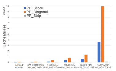Figure 10: Cache misses of parallel scoring algorithms, in billions, on Xeon4.

Table 1: Cache misses of scoring algorithms, in millions, on Xeon4. A |A| B |B| Score Diagonal Strip Imp1 Imp2 human4 97,634 mouse4 94,647 33 74 6 82.1% 92.1% XM_004403740 104,267 XM_012169741 103,004 38 86 7 81.8% 91.9% AC006294 200,000 NW_009147196 200,000 144 342 26 81.9% 92.3% AC006294 200,000 NW_004451499 398,273 363 630 52 85.6% 91.7% KQ079741 392,981 NW_004451499 398,273 712 1,190 98 86.2% 91.7% KQ079794 1,083,068 NW_004450885 1,098,196 4,676 9,200 772 83.5% 91.6% Table 2: Run time of scoring algorithms, in hh:mm:ss, on Xeon4. A |A| B |B| Score Diagonal Strip Imp1 Imp2 human4 97,634 mouse4 94,647 0:00:39 0:00:42 0:00:33 16.2% 21.6% XM_004403740 104,267 XM_012169741 103,004 0:00:45 0:00:49 0:00:38 16.2% 22.8% AC006294 200,000 NW_009147196 200,000 0:02:49 0:03:02 0:02:22 16.2% 22.1% AC006294 200,000 NW_004451499 398,273 0:05:42 0:05:58 0:04:42 17.5% 21.3% KQ079741 392,981 NW_004451499 398,273 0:11:03 0:11:44 0:09:14 16.4% 21.4% KQ079794 1,083,068 NW_004450885 1,098,196 1:24:06 1:28:45 1:10:10 16.6% 20.9%

Figure 11 and Table 5 give the running times for our parallel scoring algorithms on our Xeon4 platform. In the figure, the time is in seconds while in the table, the time is given using the format _hh : _mm : _ss. As in the table, _PP__Strip is the fastest algorithm in practice, which is up to 40_.0% faster than _PP__Score and up to 38.4% faster than PP_Diagonal.

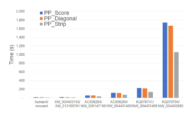Figure 11: Run time of parallel scoring algorithms, in seconds, on Xeon4.

Table 6 gives the speedup of each of our parallel scoring algorithms relative to their sequential counterparts. As can be seen, the speedup of _PP__Strip (i.e., Strip/_PP__Strip) is between 3.92 and 3.98, which is quite close to the number of cores (4) on our Xeon4 platform. _PP__Score achieves a speedup in the range

2_.82 to 2_.94 and the speedup for _PP__Diagonal is in the range 3_.12 to 3_.21.

The excellent speedup exhibited by _PP__Strip is due largely to our ability to greatly reduce cache misses for this algorithm.

Figures 12 and Tables 7 give the CPU and cache energy consumed, in joules, by our Xeon4 platform. On our datasets, _PP__Strip required up to 41_.2% less CPU and cache energy than _PP__Score and up to 45_.5% less than PP_Diagonal.

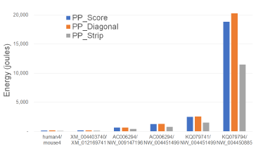Figure 12: CPU and cache energy consumption of parallel scoring algorithms, in joules, on Xeon4.

Compared to the sequential scoring algorithms, the multi-core algorithms use higher CPU power but less running time. Since the power increase is less than the decrease in running time, energy consumption is reduced.

4.2.3. Alignment Algorithms

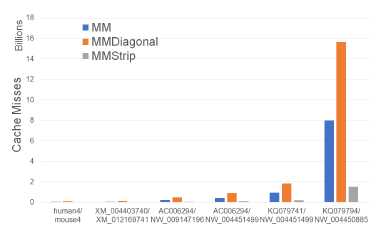Figure 13: Cache misses for alignment algorithms, in billions, on Xeon4.

Figure 13 and Table 8 give the number of cache misses of our single-core alignment algorithms on our Xeon4 plat-

Table 3: CPU and cache energy consumption of scoring algorithms, in joules, on Xeon4.

A	|A|	B	|B|	Score	Diagonal	Strip	Imp1	Imp2
human4	97,634	mouse4	94,647	230.67	252.29	190.6	17.4%	24.5%
XM_004403740	104,267	XM_012169741	103,004	268.29	297.28	221.49	17.4%	25.5%
AC006294	200,000	NW_009147196	200,000	997.88	1100.6	829.36	16.9%	24.6%
AC006294	200,000	NW_004451499	398,273	2026.26	2178.97	1651.46	18.5%	24.2%
KQ079741	392,981	NW_004451499	398,273	3944.3	4300.59	3253.46	17.5%	24.3%
KQ079794	1,083,068	NW_004450885	1,098,196	30125.93	33472.81	24980.35	17.1%	25.4%

Table 4: Cache misses of parallel scoring algorithms, in millions, on Xeon4.

A	|A|	B	|B|	PP_Score	PP_Diagonal	PP_Strip	Imp1	Imp2
human4	97,634	mouse4	94,647	34	102	1	96.7%	98.9%
XM_004403740	104,267	XM_012169741	103,004	39	115	1	96.8%	98.9%
AC006294	200,000	NW_009147196	200,000	146	398	4	96.9%	98.9%
AC006294	200,000	NW_004451499	398,273	362	768	7	98.1%	99.1%
KQ079741	392,981	NW_004451499	398,273	628	1,373	14	97.7%	99.0%
KQ079794	1,083,068	NW_004450885	1,098,196	3,642	9,976	121	96.7%	98.8%

form. _MMStrip has the fewest number of cache misses followed by MM and MMDiagonal (in this order). MMStrip reduces cache misses by up to 81_.0% relative to MM and by up to 90.3% relative to MMDiagonal. Figure 14 and Table 9 give the running times of our single-core alignment algorithms on our Xeon4 platform. As can be seen, _MMStrip is the fastest followed by MM and MMDiagonal (in this order). MMStrip reduces running time by up to 15_.0% relative to _MM, by up to 13_.4% relative to _MMDiagonal. As was the case with our scoring algorithms, the reduction in running time, while significant, isn’t as much as the reduction in cache misses.

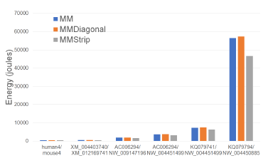Figure 15: CPU and cache energy consumption of alignment algorithms, in joules, on Xeon4.

Figures 15 and Tables 10 give the CPU and cache energy consumption, in joules, by our single-core alignment algorithms. On our datasets, _MMStrip reduced

up to 17_.5% less CPU and cache energy than _MM Figure 16: Cache misses for parallel alignment algoand up to 18.7% less than MMDiagonal. Once again, rithms, in billions, on Xeon4.

the energy reduction is comparable to the reduction in running time suggesting a close relationship between _PP__MMStrip has the fewest number of cache running time and energy consumption for this applica- misses followed by _PP__MM and _PP__MMDiagonal tion. (in this order). _PP__MMStrip reduces cache misses by Table 5: Run time of parallel scoring algorithms on Xeon4.

A	|A|	B	|B|	PP_Score	PP_Diagonal	PP_Strip	Imp1	Imp2
human4	97,634	mouse4	94,647	0:00:14	0:00:13	0:00:08	40.0%	37.7%
XM_004403740	104,267	XM_012169741	103,004	0:00:16	0:00:15	0:00:10	39.8%	37.1%
AC006294	200,000	NW_009147196	200,000	0:00:58	0:00:58	0:00:36	39.0%	38.4%
AC006294	200,000	NW_004451499	398,273	0:01:56	0:01:53	0:01:11	39.0%	37.0%
KQ079741	392,981	NW_004451499	398,273	0:03:49	0:03:39	0:02:19	39.3%	36.6%
KQ079794	1,083,068	NW_004450885	1,098,196	0:29:02	0:27:52	0:17:39	39.2%	36.7%

Table 6: Speedup of parallel scoring algorithms on Xeon4.

A	|A|	B	|B|	Score/PP	Diagonal/PP	Strip/PP
human4	97,634	mouse4	94,647	2.82	3.12	3.93
XM_004403740	104,267	XM_012169741	103,004	2.82	3.19	3.92
AC006294	200,000	NW_009147196	200,000	2.89	3.14	3.97
AC006294	200,000	NW_004451499	398,273	2.94	3.18	3.97
KQ079741	392,981	NW_004451499	398,273	2.89	3.21	3.98
KQ079794	1,083,068	NW_004450885	1,098,196	2.90	3.18	3.98

up to 95_.5% relative to _PP__MM and by up to 98_.2% relative to PP_MMDiagonal.

Figure 17 and Table 12 give the running times for our parallel alignment algorithms on the Xeon4 platform. PP_MMStrip is faster than PP_MM by up to 37.4% and faster than PP_MMDiagonal by up to

40.3%.

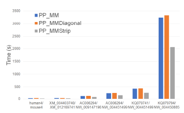Figure 17: Run time of parallel alignment algorithms, in seconds, on Xeon4.

Table 13 gives the speedup of each parallel alignment algorithm relative to its single-core counterpart.

The speedup achieved by _PP__MMStrip (relative to MMStrip) ranges from 3.56 to 3.94 while that for PP__MM is in the range 2.77 to 2.88 and that for PP_MMDiagonal is in the range 2.53 to 2.81.

Figures 18 and Tables 14 give the CPU and cache energy consumption, in joules, by our multi-core alignment algorithms. On our datasets, _PP__MMStrip required up to 29_.9% less CPU and cache energy than _PP__MM and up to 42.1% less than PP_MMDiagonal. Once again, the energy reduction is comparable to the reduction in running time suggesting a close relationship between running time and energy consumption for this application.

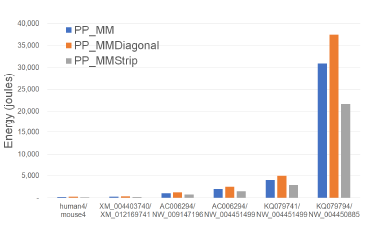Figure 18: CPU and cache energy consumption of parallel alignment algorithms, in joules, on Xeon4.

4.3. I7-x980 (Xeon6)

4.3.1. Scoring Algorithms

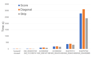Figure 19: Run time of scoring algorithms, in seconds, on Xeon6

Figure 19 and Table 15 give the running times of our single-core scoring algorithms on our Xeon6 platform. As can be seen, _Strip is the fastest followed by _Score and _Diagonal (in this order). _Strip reduces running time by up to 14_.3% relative to _Score and by up to 22.4% relative to Diagonal.

Table 7: CPU and cache energy consumption of parallel scoring algorithms on Xeon4. A |A| B |B| PP_Score PP_Diagonal PP_Strip Imp1 Imp2 human4 97,634 mouse4 94,647 150.12 161.77 88.23 41.2% 45.5% XM_004403740 104,267 XM_012169741 103,004 174.30 175.68 102.76 41.0% 41.5% AC006294 200,000 NW_009147196 200,000 631.46 661.29 381.02 39.7% 42.4% AC006294 200,000 NW_004451499 398,273 1,256.11 1,294.55 760.57 39.5% 41.2% KQ079741 392,981 NW_004451499 398,273 2,471.51 2,535.50 1,493.38 39.6% 41.1% KQ079794 1,083,068 NW_004450885 1,098,196 18,830.03 20,253.39 11,477.30 39.0% 43.3% Table 8: Cache misses for alignment algorithms, in millions, on Xeon4. A |A| B |B| MM MMDiagonal MMStrip Imp1 Imp2 human4 97,634 mouse4 94,647 42 96 12 71.6% 87.6% XM_004403740 104,267 XM_012169741 103,004 54 119 14 74.5% 88.5% AC006294 200,000 NW_009147196 200,000 227 488 48 78.6% 90.1% AC006294 200,000 NW_004451499 398,273 441 926 95 78.4% 89.7% KQ079741 392,981 NW_004451499 398,273 959 1,851 200 79.1% 89.2% KQ079794 1,083,068 NW_004450885 1,098,196 7,994 15,642 1,521 81.0% 90.3%

4.3.2. Parallel Scoring Algorithms

Figure 20 and Table 16 give the running times for our parallel scoring algorithms on our Xeon6 platform. As with Xeon4, PP_Strip is faster than PP_Score and PP__Diagonal and reduces the running time by up to 42_.5% and 55_.6%, respectively.

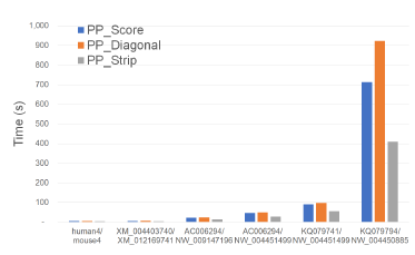Figure 20: Run time of parallel scoring algorithms, in seconds, on Xeon6.

Table 18 gives the speedup of each of our parallel algorithms relative to their single-core counterparts. PP__Strip achieves a speedup of up to 5_.89, which is very close to the number of cores. The maximum speedup achieved by PP_Score and PP_Diagonal was 4_.09 and 4_.25, respectively.

4.3.3.  Alignment Algorithms

Figure 21 and Table 17 give the running times of our parallel scoring algorithms on the Xeon6 platform. As can be seen, _MMStrip is the fastest followed by _MM and MMDiagonal (in this order). MMStrip reduces running time by up to 12_.6% relative to _MM and by up to 14.2% relative to MMDiagonal.

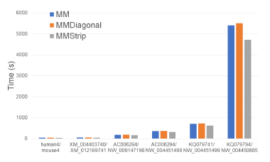Figure 21: Run time of alignment algorithms, in seconds, on Xeon6.

4.3.4. Parallel Alignment Algorithms

Figure 22 and Table 20 give the running times of our parallel alignment algorithms on the Xeon6.

PP_MMStrip is faster than PP_MM and PP_MMDiagonal and reduces the running time by up to 39_.9% and 44_.8%, respectively.

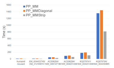Figure 22: Run time of parallel alignment algorithms, in seconds, on Xeon6.

Table 9: Run time of alignment algorithms on Xeon4. A |A| B |B| MM MMDiagonal MMStrip Imp1 Imp2 human4 97,634 mouse4 94,647 0:01:12 0:01:13 0:01:03 12.6% 12.7% XM_004403740 104,267 XM_012169741 103,004 0:01:27 0:01:24 0:01:14 15.0% 12.8% AC006294 200,000 NW_009147196 200,000 0:05:16 0:05:14 0:04:33 13.6% 13.0% AC006294 200,000 NW_004451499 398,273 0:10:25 0:10:18 0:09:04 13.0% 12.0% KQ079741 392,981 NW_004451499 398,273 0:20:27 0:20:28 0:17:47 13.0% 13.1% KQ079794 1,083,068 NW_004450885 1,098,196 2:36:12 2:35:53 2:14:59 13.6% 13.4% Table 10: CPU and cache energy consumption of alignment algorithms on Xeon4. A |A| B |B| MM MMDiagonal MMStrip Imp1 Imp2 human4 97,634 mouse4 94,647 426.38 438.07 369.94 13.2% 15.6% XM_004403740 104,267 XM_012169741 103,004 509.66 511.32 431.59 15.3% 15.6% AC006294 200,000 NW_009147196 200,000 1873.99 1911.35 1600.77 14.6% 16.2% AC006294 200,000 NW_004451499 398,273 3707.55 3772.38 3189.38 14.0% 15.5% KQ079741 392,981 NW_004451499 398,273 7313.49 7512.26 6278.63 14.2% 16.4% KQ079794 1,083,068 NW_004450885 1,098,196 56478.59 57339.29 46589.55 17.5% 18.7%

Table 21 gives the speedup of each of our parallel algorithms relative to their single-core counterparts. _PP__MMStrip achieves a speedup of up to 5_.78, which is very close to the number of cores.

The maximum speedup achieved by _PP__MM and PP_MMDiagonal was 3.98 and 3.80, respectively.

4.4.  Xeon E5-2695 (Xeon24)

4.4.1. Scoring Algorithms

Figure 23 and Table 19 give the running times of our single-core scoring algorithms on our Xeon24 platform. As was the case on our other test platforms, _Strip is the fastest followed by _Score and _Diagonal (in this order). Strip reduces running time by up to 19_.7% relative to Score and by up to 35.1% relative to Diagonal.

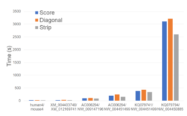Figure 23: Run time of scoring algorithms, in seconds, on Xeon24.

4.4.2. Parallel Scoring

Algorithms Figure 24 and Table 22 give the running times for our parallel scoring algorithms on our Xeon24 platform. PP_Strip is faster than PP_Score and PP__Diagonal and reduces the running time by up to 61_.4% and 76_.2%, respectively.

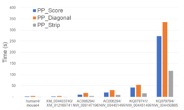Figure 24: Run time of parallel scoring algorithms, in seconds, on Xeon24.

Table 23 gives the achieved speedup. _PP__Strip scales quite well and results in a speedup of up to 22.22.

The maximum speedups provided by _PP__Score and PP__Diagonal are 11.36 and 9.56, respectively.

4.4.3. Alignment Algorithms

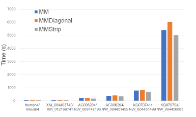Figure 25: Run time of alignment algorithms, in seconds, on Xeon24.

Figure 25 and Table 24 give the running times of our single-core alignment algorithms on our Xeon24 plat-

Table 11: Cache misses for parallel alignment algorithms, in millions, on Xeon4. A |A| B |B| PP_MM PP_MMDiagonal PP_MMStrip Imp1 Imp2 human4 97,634 mouse4 94,647 64 137 9 85.3% 93.1% XM_004403740 104,267 XM_012169741 103,004 71 161 17 75.8% 89.4% AC006294 200,000 NW_009147196 200,000 251 625 23 91.0% 96.4% AC006294 200,000 NW_004451499 398,273 495 1,296 39 92.2% 97.0% KQ079741 392,981 NW_004451499 398,273 975 2,558 52 94.6% 98.0% KQ079794 1,083,068 NW_004450885 1,098,196 7,001 17,721 314 95.5% 98.2% Table 12: Run time of parallel alignment algorithms on Xeon4. A |A| B |B| PP_MM PP_MMDiagonal PP_MMStrip Imp1 Imp2 human4 97,634 mouse4 94,647 0:00:26 0:00:29 0:00:17 34.5% 40.3% XM_004403740 104,267 XM_012169741 103,004 0:00:30 0:00:33 0:00:21 31.6% 37.3% AC006294 200,000 NW_009147196 200,000 0:01:52 0:01:56 0:01:12 36.1% 38.5% AC006294 200,000 NW_004451499 398,273 0:03:43 0:03:50 0:02:20 37.4% 39.1% KQ079741 392,981 NW_004451499 398,273 0:07:12 0:07:23 0:04:31 37.2% 38.8% KQ079794 1,083,068 NW_004450885 1,098,196 0:54:03 0:55:33 0:34:20 36.5% 38.2%

form. _MMStrip is the fastest followed by _MM and MMDiagonal (in this order). MMStrip reduces running time by up to 17_.1% relative to _MM and by up to 16.8% relative to MMDiagonal.

4.4.4. Parallel Alignment Algorithms

Figure 26 and Table 25 give the running times of our parallel alignment algorithms on Xeon24. As can be seen, PP_MMStrip is faster than PP_MM and PP_MMDiagonal. It reduces the running time by up to 47_.3% and 84_.6%, respectively.

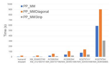Figure 26: Run time of parallel alignment algorithms, in seconds, on Xeon24.

Table 26 gives the speedup of our parallel algorithms. _PP__MMStrip achieves a speedup of up to 16.2 while PP_MM and PP_MMDiagonal have maximum speedups of 9.79 and 6.58.

5. Discussion

By accounting for the presence of caches in modern computers, we are able to arrive at sequence alignment algorithms that are considerably faster than those that do not take advantage of computer caches. Our benchmarking demonstrates the value of optimizing cache usage. Our cache-efficient algorithms _Strip and MMStrip were the best-performing single-core algorithms and their parallel counterparts were the bestperforming parallel algorithms. _Strip reduced running time by as much as 19_.7% relative to the classical scoring algorithm _Score due to Smith and Waterman and

MM__Strip reduced running time by as much as 17_.1% relative to the alignment algorithm of Myers and Miller. Neither the algorithm of Smith and Waterman nor that of Myers and Miller optimize cache utilization. The parallel versions of _Strip and _MM__Strip were up to 61_.4% and 47_.3% faster than the parallel versions of the Smith and Waterman and the Myers and Miller algorithms, respectively.

6. Limitations

Our cache miss analyses assume a simple cache model in which there is a single LRU cache. In practice, computers have multiple levels of cache and employ sophisticated and proprietary cache replacement strategies. Despite the use of a simplified cache model for analysis, the developed cache-efficient algorithms perform very well in practice.

7. Conclusion

The main contributions of this papers are

1. cache efficient single-core and multi-core algorithms to determine the score of the best alignment;
2. cache efficient single-core and multi-core algorithms to determine the best alignment.

The effectiveness of our cache-efficient algorithms has been demonstrated experimentally using three computational platforms. Future work includes developing the cache-efficient algorithms for other problems in computational biology.

Conflict of Interest The authors declare no conflict of interest.

Table 13: Speedup of parallel alignment algorithms on Xeon4.

A	|A|	B	|B|	MM/PP	MMDiagonal/PP	MMStrip/PP
human4	97,634	mouse4	94,647	2.77	2.53	3.70
XM_004403740	104,267	XM_012169741	103,004	2.78	2.56	3.56
AC006294	200,000	NW_009147196	200,000	2.80	2.70	3.81
AC006294	200,000	NW_004451499	398,273	2.84	2.69	3.89
KQ079741	392,981	NW_004451499	398,273	2.84	2.78	3.94
KQ079794	1,083,068	NW_004450885	1,098,196	2.88	2.81	3.93

Table 14: CPU and cache energy consumption of parallel alignment algorithms on Xeon4.

A	|A|	B	|B|	PP_MM	PP_MMDiagonal	PP_MMStrip	Imp1	Imp2
human4	97634	mouse4	94647	236.98	305.14	181.6	23.4%	40.5%
XM_004403740	104267	XM_012169741	103004	272.26	352.56	216.83	20.4%	38.5%
AC006294	200000	NW_009147196	200000	1044.86	1279.77	747.86	28.4%	41.6%
AC006294	200000	NW_004451499	398273	2039.55	2540.52	1483.8	27.2%	41.6%
KQ079741	392981	NW_004451499	398273	4020.48	4979.17	2905.32	27.7%	41.7%
KQ079794	1083068	NW_004450885	1098196	30964.02	37461.35	21703.65	29.9%	42.1%

Acknowledgment

This work was supported, in part, by the National Science Foundation under award NSF 1447711.

1. Henikoff and J. G. Henikoff, “Amino acid substitution matrices from protein blocks,” Proc Natl Acad Sci U S A, vol. 89, pp. 10 915–10 919, 1992.
2. B. Needleman and C. D. Wunsch, “A general method applicable to the search for similarities in the amino acid sequence of two proteins,” Journal of Molecular Biology, vol. 48, pp. 443–453, 1970.
3. F. Smith and M. S. Waterman, “Identification of common molecular subsequences,” Journal of Molecular Biology, vol. 147, pp. 195–197, 1981.
4. Gotoh, “An improved algorithm for matching biological sequences,” Journal of Molecular Biology, vol. 162, pp. 705–708, 1982.
5. S. Hirschberg, “A linear space algorithm for computing longest common subsequences,” Communications of the ACM, vol. 18, pp. 341–343, 1975.
6. Myers and W. Miller, “Optimal alignments in linear space,” Computer Applications in the Biosciences(CABIOS), vol. 4, pp. 11–17, 1988.
7. Huang, R. Hardison, and W. Miller, “A space-efficient algorithm for local similarities,” Comput Appl Biosci, vol. 6, p. 373âAS381, 1990.
8. Altschul, W. Gish, W. Miller, E. Myers, and D. Lipman, “Basic local alignment search tool,” Journal of Molecular Biology, vol. 215, pp. 403–410, 1990.
9. Pearson and D. Lipman, “Improved tools for biological sequence comparison,” Proceedings of the National Academy of Sciences USA, vol. 85, pp. 2444–2448, 1988.
10. Chao, J. Zhang, J. Ostell, and W. Miller, “A local alignment tool for very long dna sequences,” Comput Appl Biosci, vol. 11, pp. 147–153, 1995.
11. Driga, P. Lu, J. Schaeffer, D. Szafron, K. Charter, and I. Parsons, “Fastlsa: a fast, linear-space, parallel and sequential algorithm for sequence alignment,” Algorithmica, vol. 45, p. 337âAS375, 2006.
12. Li, S. Ranka, and S. Sahni, “Pairwise sequence alignment for very long sequences on gpus,” IEEE 2nd International Conference on Computational Advances in Bio and Medical Sciences (ICCABS), 2012.
13. O. Sandes and A. C. M. A. Melo, “Smith-waterman alignment of huge sequences with gpu in linear space,” IEEE International Symposium on Parallel and Distributed Processing (IPDPS), pp. 1199–1211, 2011.
14. Aluru and N. Jammula, “A review of hardware acceleration for computational genomics,” IEEE Design and Test, vol. 31, pp. 19–30, 2014.
15. Rajko and S. Aluru, “Space and time optimal parallel sequence alignments,” IEEETPDS:IEEE Transactions on Parallel and Distributed Systems, vol. 15, 2004.
16. Khajeh-Saeed, S. Poole, and J. B. Perot, “Acceleration of the smithâASwaterman algorithm using single and multiple graphics processors,” Journal of Computational Physics, p. 4247âAS4258, 2010.
17. Kurtz, A. Phillippy, A. L. Delcher, M. Smoot, M. Shumway, C. Antonescu, and S. L. Salzberg, “Versatile and open software for comparing large genomes,” Genome Biol, vol. 5, 2004.
18. Almeida and N. Roma, “A parallel programming framework for multi-core dna sequence alignment,” Complex, Intelligent and Software Intensive Systems (CISIS), 2010 International Conference on, pp. 907 – 912, 2010.
19. Hamidouche, F. M. Mendonca, J. Falcou, A. C. M. A. Melo, and D. Etiemble, “Parallel smith-waterman comparison on multicore and manycore computing platforms with bsp++,” International Journal of Parallel Programming, vol. 41, pp. 1110–136, 2013.
20. Zhao and S. Sahni, “Cache and energy efficient alignment of very long sequences,” 2015 IEEE 5th international conference on Computational Advances in Bio and Medical Sciences (ICCABS), 2015.
21. “Perf tool,” https://perf.wiki.kernel.org/index.php/ Main_Page.
22. “Globin gene server,” http://globin.cse.psu.edu/globin/ html/pip/examples.html.
23. “Ncbi database,” http://www.ncbi.nlm.nih.gov/gquery.

(Click Here)

(Click Here)