1. Introduction

Nowadays significant amount of energy is consumed in commercial or residential buildings by the heating, ventilation and air conditioning (HVAC) systems to provide thermally comfortable indoor environment. Consequently, improving their efficiency becomes a critical issue for energy and environmental sustainability. In most commercial buildings, chilled-water from centrifugal chillers is supplied to air-handling units to meet the cooling needs of the building. The overall system as shown in Figure 1 consists of two water circuits: in one circuit water is circulated through the evaporator to produce chilled water and the second water circuit is used to reject heat to outdoors through a cooling tower [1-7]. During the last two decades, for a wide variety of HVAC control systems applications, the centrifugal chillers have become the most widely used due to their high capacity, high reliability, and low maintenance [7]. Moreover, among the major devices in chilled-water systems, the centrifugal chiller is the most energy-consuming device, and its efficiency can be improved by implementing advanced model-based controller design strategies and fault detection and isolation (FDI) methodologies.

 Consequently, the development of high-fidelity dynamic centrifugal chiller models has become a priority task of our research. A brief literature review in this field reveals that a significant amount of work has been done on transient and steady state modeling for centrifugal chillers [1]-[4], [7-11].

 On the other hand, several dynamic models for vapor compression cycle also have been extensively studied, such as in [6] where is modeled a reciprocating compressor with polytrophic efficiency, that includes also a compressor housing and refrigerant mixing with the oil in the sump. The heat exchanger is modeled based on moving boundary method that assumes an average state for each phase region according to well mixed modeling assumption. The expansion valve is modeled based on isenthalpic process, and in addition the dynamics of the sensing bulb is also considered. The simulation models are tested with shut-down and start-up and different operations.  An interesting approach we find in [9] where a centrifugal compressor model is developed based on control volume methodology that designs the impeller and diffuser separately as control volumes; the impeller is modeled in detail based on the Euler equations, and the diffuser is modeled as ideal without any losses.  The mass flow rate and the exit state enthalpy specific for low pressure refrigerant R234a are predicted by two empirical relations. A substantial improvement of this model we find in [10], where a liquid chiller lumped – parameter model of the heat exchangers is developed. Input step changes in the condenser-side water flow rates are studied in order to simulate the system performance under disturbances. Furthermore, in [8] is developed a mechanistic, single stage and two-stage centrifugal chiller models where the centrifugal compressor is modeled based on the Euler turbo-machinery theory, the energy balance and the impeller velocity equations. The coefficient of performance (COP) of the chiller is simulated by considering the compressor polytropic efficiency, hydrodynamic, mechanical and electrical losses. On the other hand, the condenser and evaporator are modeled based on lumped parameter approach and the heat transfer is calculated based on effectiveness model. The chiller model is validated with a water-to-water chiller test facility. The simulations reveal that the chiller dynamic model predicts higher start-up condenser and evaporator pressures than the measurements, more precisely the modeled dynamics seems to appear faster than the experiment results for convergence to the steady-state. Also, the evaporator-side model performs better than the condenser-side in terms of predicting the transient responses. In an another study [2] a dynamic centrifugal liquid chiller model with flooded-type shell-and-tube heat exchangers is developed, where the compressor model is based on a constant speed and its capacity control is achieved by variable inlet guide vane (IGV). An interesting regression model was applied in [8] to determine the maximum capacity condition, i.e., with wide-open IGV, and the actual mass flow rate was then computed based on a linear relationship of the maximum mass flow rate and the IGV position.

 During the transient periods, in a numerical simulation environment was found the optimal values of the initial and the overall system charges. Moreover in [8] is mentioned that for simulations purpose, due to complex nature of the refrigeration cycle, it seems that all the existing simulation models developed for centrifugal chillers include some simplifications for some components. For the centrifugal compressor, the dynamic performance was often approximated based on the compressor characteristic map rather than parameterized dynamic models as is mentioned in [1, 4, 6]. Such approximation is sufficient for simulating the steady-state performance of the chiller, whereas may lead to difficulty in simulating transient processes such as startup, load change and shutdown. In [11] is developed a dynamic model for the centrifugal compressor where the model of the heat exchangers is based on lumped parameters approach.

 The objective of our research is to develop a comprehensive dynamic model for the centrifugal chiller suitable for control analysis and design. In particular we aim to achieve quality simulation performance in MATLAB and SIMULINK modeling, and simulations environment for all components of centrifugal chiller. The significance of the proposed research includes the following:

• The dynamic characteristics of the centrifugal chiller system was modeled based on detailed mass, momentum and energy balance equations
• The shell-and-tube heat exchangers were modeled based on lumped parameters approach.
• The developed control strategies based on the centrifugal chiller model cover different operating conditions in order to be robust to several changes of the parameters control structure or modeling errors, and to achieve the best transient and steady-state performance.

In this paper we are focused to get accurate models for centrifugal chiller and based on these models to develop a few PI closed-loop control strategies to find the most suitable control strategy for these kinds of applications that performs better in terms of accuracy, robustness, convergence speed, overshoot, and disturbance rejection. The performance comparison of the proposed control strategies is very useful to choose the most suitable control strategy that performs better in terms of meeting the control design requirements and process control constraints, rejection of the effect of possible disturbances that act on the controlled process, as well as a tracking error accuracy.

2. The Centrifugal Chiller Nonlinear Model

2.1.  Modeling and description of components

In Figure 1 is shown a schematic of the water-cooled centrifugal chiller system which consists of four major components: a centrifugal compressor, an expansion valve, an evaporator, and a condenser [8]. In general, the overall chilled-water system consists of one circuiting refrigerant loop and two water loops. The first water loop is circuited between the condenser and the cooling tower, and the second water loop is circuited between the evaporator and the air handling unit (AHU). In our research, a detailed nonlinear model of a centrifugal chiller system is developed. The modeling methodology and the model equations are described in Annex-1 appended at the end of this paper. The nonlinear model consists of four major sub-component models, namely, a flooded evaporator, a flooded water-cooled condenser, a centrifugal compressor and an electronic expansion valve. The simulation of transient and steady-state behavior of the water-cooled centrifugal chiller is performed in a well-known MATLAB / SIMULINK environment. As described in Annex-1, the dynamic model of the overall centrifugal chiller system is of high complexity in terms of state dimension and nonlinearity. The nonlinear model equations were then reformulated into a state space model by a set of 40 first order differential equations (ODE), as a mathematical form to represent the physical chiller system.

 The significant aspects of the nonlinear model are presented briefly in this section.

First, we focus our attention to centrifugal compressor that is the much faster responding device in the chiller plant. Similar as is shown in [8] the centrifugal compressor capacity balance is achieved with variable rotor speed control. In our research, the capacity control is manipulated by adjusting the IGV position and input torque, as shown in Figure 2. The model takes into account also, the effects of incidence and fluid friction losses, mentioned in [8].  Figure 2 schematically depicts the centrifugal model with boundary conditions and capacity control. It is important to note that the working medium in the centrifugal chillers is refrigerant that works under multi-phase conditions, which makes it more complex and difficult for the underlying modeling framework and consistent numerical initialization [8].

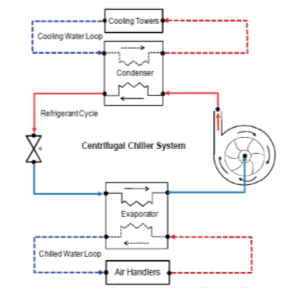Figure 1. Schematic of water-cooled centrifugal chiller system (see [8])

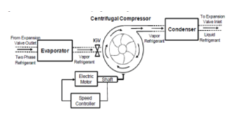Figure 2. The schematic of the centrifugal compression system in chiller (see [8])

The evaporator and condenser modeling requires quality heat exchanger models. The flooded evaporator was divided into a two-phase section and a superheat section as detailed in Annex-1. Likewise, the flooded condenser was divided into two superheat sections, a two-phase section and a sub-cool section.

The electronic expansion valve (EXV) was modeled to regulate the flow rate of refrigerant in the system and in this study the EXV was used to maintain the liquid level of the refrigerant in the condenser. The modeling details are described in Annex-1.

The dynamic model for centrifugal chiller system presented in Annex-1 is reformulated in state-space representation, by a linear set of ordinary differential equations (ODE), as a natural representation of a physical system, and easily to be solved using a suitable MATLAB solver.

3. MATLAB Open-Loop Simulation results

Simulations were performed with the nonlinear centrifugal chiller model to investigate its open-loop dynamic behavior and steady-state performance using R134a as refrigerant, in a MATLAB/SIMULINK simulation environment.  In open-loop the centrifugal chiller is a multi-input, multi-output (MIMO) control system that has two inputs, namely the  compressor motor drive speed (Ucom),  and the expansion valve opening (U_EXV),  two outputs corresponding to chilled water temperature (Tchwsp), and the liquid level in condenser (Level)). Using a consistent set of initial conditions, simulation runs were conducted under constant design load conditions. The open-loop simulation results are shown in Figure 3.  The temperature and pressure responses are smooth and reach their respective design operating conditions as the system reaches steady state. The responses in Figure 3 depict the condensing pressure Pc in 3(a), the evaporation pressure Pev in 3(b), chilled water temperature (Tchw,sp) in 3(c), water temperature in the condenser 3(d),  the heat exchange rate in 3(e) and the coefficient of performance in 3(f).  From these results it can be noted that the system responses reach steady state in about 30 minutes when subjected to constant load. At steady state the coefficient of performance of the system is 5.5 and the heat rejection rate is about 20% greater than the cooling capacity as a result of heat generated by the compressor motor.

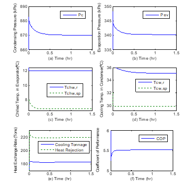Figure 3.  Open-loop responses of the chiller system

Legend: (a) Compression pressure (Pc); (b) Evaporation pressure (Pev); (c)Chilled water temperature Tchw, sp; (d) Water temperature in condenser Tcw; (e) Cooling tonnage and heat rejection; (f) Coefficient of performance (COP);

The SIMULINK model of centrifugal chiller system in open-loop and its details are shown in Figures 4 and 5. These figures with higher resolution are also depicted in Annex-2.

The MATLAB Function1 in the SIMULINK model from Figure 5 has the following code lines:

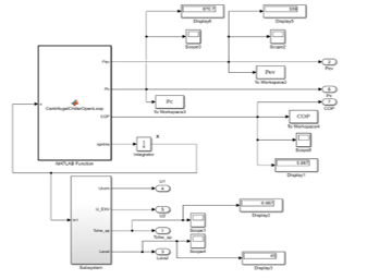Figure 4: The SIMULINK model of centrifugal chiller in open-loop

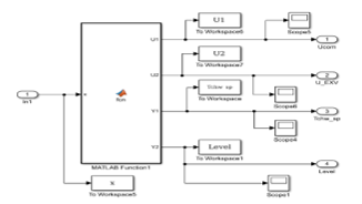Figure 5. The SIMULINK model of the bottom Subsystem Block

The Centrifugal Chiller open-loop model is very useful to build the PI control strategy as described in the next section for the overall system seen as centralized system, since in “real-life” there exist some interferences between the loops. Furthermore, through open-loop simulations we generate sets of input-output data required to build the ARMAX models for Centrifugal chiller. This is the reason to start with a good open-loop model capable to capture entire dynamics of the overall chiller system under various operating conditions. This give us more flexibility for control design.

4. Closed – Loop Control Strategies Design

In this section we develop and implement in a MATLAB/SIMULINK environment three closed-loop control strategies, namely an overall Proportional-Integral (PI) controller based on the chiller system model in open-loop developed and implemented in MATLAB simulation environment in previous section 3. By extensive simulations we found that the interference between the both loops, temperature and liquid Refrigerant level, respectively, is very week, and thus we can simplify the overall chiller system model by considering that the loops are decoupled.

 This is an essential modeling aspect that is investigated in this research paper, by building for each loop separately a PI controller, as is developed in subsection 4.1. The SIMULINK model of PI controllers for each separate loop is shown in Annex-2.

 The open-loop model is useful also to generate the set of input-output data measurements necessary to build the linear ARMAX SISO models. The input-output data set measurements file was loaded in a new MATLAB code file that estimates the ARMAX SISO models.

However, from accuracy considerations, in the future research work we will investigate also the extension of ARMAX multi-input single output (MISO) models for building predictive control strategies. In subsection 4.2 the ARMAX SISO decoupled models will be used to build one linear PI controller for each loop separately.  The third control strategy is an improved PI control version that is conceived within the context of non-minimum state space control system. The non-minimal state space representation in contrast to minimal state space realizations “seems to be the natural description of a discrete-time transfer function, since its dimension is dictated by the complete structure of the model”, as is mentioned in [12-16]. More precisely, we talk about on improved version of Proportional – integral control, so called Proportional-integral-plus (PIP) control for systems with time delay [12-16], that is developed in subsection 4.3. Based on ARMAX models is proved also the superiority of new PPI controller compared with the first two PI  versions in terms of efficiency, implementation simplicity, convergence speed and robustness to the load changes disturbance and to the changes in the noise level of measurement sensors. It is worth to mention again the particular structure for this kind of applications of   the MIMO centrifugal chiller control system to be split into two single input-single output (SISO) independent closed – loops control subsystems (i.e. the  Evaporator chilled water temperature loop to control the Tchwsp, and the Condenser liquid Refrigerant level  loop  to control the Refrigerant liquid Level. The preset values of the first closed-loop is Tchw_set = 6.67 [°C], and for the second closed-loop is Level set = 45(%) of the maximum level of the liquid Refrigerant inside the Condenser.  Also, a PIP closed-loop control is developed in detail in subsection 4.3. Concluding, at the end of section 4 we can decide on a potential controller choice amongst these three control strategies to find the one that performs better in terms of the accuracy, robustness to the changes in the load magnitude, considered as a disturbance, and to the level of measurement noises injected additionally in each forward loop to Tchwsp, and to liquid Level respectively.

4.1. Closed-loop PI Control Strategy of MIMO

4.2. Centrifugal Chiller System

In this subsection we design for each open-loop a PI control strategy given by [12-16]:

• closed-loop PI control strategy of chilled water temperature Tchwsp of Evaporator:

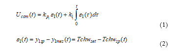where  is the error between the set point value of the closed-loop output temperature  value and its measured value ; , are the tuning proportional, integral coefficients of the first PI controller.

• closed-loop PI control strategy of liquid level inside the condenser:

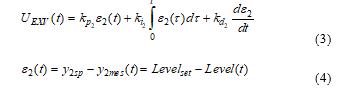where is the error between the set point value of the closed-loop output liquid level value and its measured value ; , are the tuning proportional, integral coefficients of the second PI controller.

An extensive number of simulations for adjusting the coefficients of both PI controllers in order to perform well in terms of overshoot, settling time and steady-state error led to the following values:

• For closed-loop Evaporator subsystem:

i.e. the Temperature set-point value.

• For closed-loop Condenser subsystem

, i.e. the Liquid level setting point value.

The closed-loop simulation results related to PI controller performance for Evaporator subsystem are shown in Figure 6 for Condenser subsystem, and in Figure 7 they are related to the overall performance in terms of coefficient of performance COP of entire MIMO control system. In Figure 6 are shown the chilled water Evaporator temperatures (Tchwsp, Tchwsp_set) as in 6(a), the evaporation pressure Pev in 6(b), and the Compressor motor speed actuator efforts in 6(c).

In Figure 7 is showing the PI controller closed-loop performance for Condenser subsystem related to the Refrigerant liquid level, such in 7(a), condensing pressure Pc as is revealed in 7(b), and expansion valve actuator effort presented in 7(c).

The overall performance for entire MIMO control system in the particular case of nonlinear plant dynamics in terms of coefficient of performance is shown in Figure 8.

Concluding, in this section we can see that the closed-loop PI controller of Condenser subsystem perform better compared to the closed-loop PI controller of Evaporator subsystem in terms of accuracy, fast transient, and disturbance rejection, as is shown in Figure 9 for the Evaporator chilled water temperature, and in  Figure 10 for Refrigerant liquid level in the  Condenser.

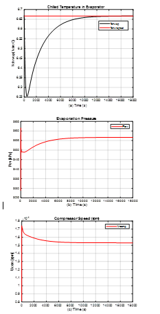Figure 6. PI control strategy for closed-loop simulations for chiller plant model- Evaporator Subsystem

Legend: (a) Temperature water supply pressure Tchwsp; (b) Evaporation pressure Pev; (c) Compressor motor drive actuator speed

As disturbance, is considered a sharp variation of the load, i.e. the temperature of chilled water Tchw_rr that increases from 48[°C] to 52[°C]), injected inside the MIMO control system by addition in the forward path of the chilled water temperature of Evaporator subsystem before the measured chilled water temperature output, after 9000 seconds (2 hours and 30 minutes), persisting further 2 hours and 30 minutes. This time assures for MIMO control system enough time to reach a new steady-state.

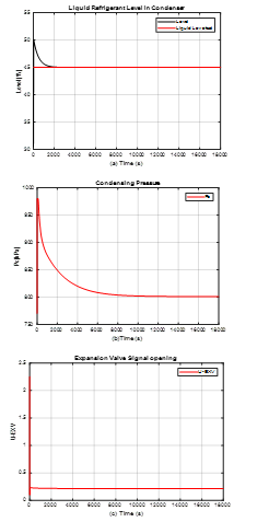Figure 7. PI control strategy for closed-loop simulations for chiller plant model – Condenser Subsystem

Legend: (a) Refrigerant liquid level; (b) Condensing pressure Pc; (c) Expansion valve actuator opening

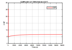Figure 8 Overall coefficient of performance COP

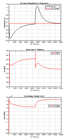Figure 9. PI control strategy for closed-loop simulations for chiller plant model – Evaporator subsystem, disturbance rejection

Legend: (a) Temperature water supply pressure Tchwsp; (b) Evaporation pressure Pev; (c) Compressor motor drive actuator speed

The both PI controllers perform very well and prove a good robustness to the changes in the control system load, with a significant amount effort of both actuators, especially by the compressor motor drive. The SIMULINK models of both PI control strategies are attached for clearness in the Annex-2. The simulation results reveal also that the PI controller of the Refrigerant liquid level in Condenser subsystem compared to PI controller of the Evaporator subsystem performs faster, during a very short transient time to reject the disturbance impact, therefore is more robust. Despite the changes in the load is worth to mention that the coefficient of performance for entire MIMO control system, as is shown in Figure 11, changes smoothly and regains in short time the optimal value reached in steady-state before the disturbance injection.

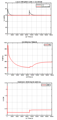Figure 10. PI control strategy for closed-loop simulations for chiller plant model – Condenser subsystem, disturbance rejection

Legend: (a) Refrigerant liquid level; (b) Condensing pressure Pc; (c) Expansion valve actuator opening U_EXV

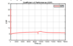Figure 11. Robustness of the overall coefficient of performance COP to a sharp disturbance variation in the load

Additionally, a normally distributed Gaussian random signal is injected in the output chilled water temperature loop and Refrigerant liquid level loop in order to simulate the impact of the measurement noise level. For a variance in measurement noise level of 0.0001 in chilled water temperature, and 0.1 in the Refrigerant liquid level, their impact on the both PI controllers performance are shown in Figure 12 and Figure 13. The simulation results shown in Figure 13 reveal a good behavior of the closed-loop PI controller of the Refrigerant liquid level compared to closed-loop PI controller of chilled water temperature.

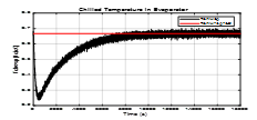Figure 12. Tchwsp – Measurement noise impact on the MIMO control system response (noise level variance 0.001)

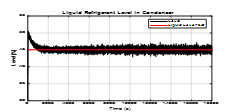Figure 13. Refrigerant liquid level – Measurement noise on the MIMO control system response (noise level variance 0.1)

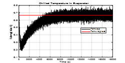Figure 14 Tchwsp – Measurement noise impact on the MIMO control system response (noise level variance increased to 0.001)

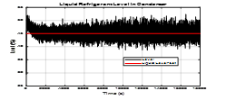Figure 15. Refrigerant liquid level – Measurement noise impact on the MIMO control system response (noise level variance increased to 1)

The impact due to ten times rise in the measurement noise levels becomes significant, as is shown in Figure 14, and Figure 15. The simulation results reveal a fragile robustness of the both PI controllers to changes in noise variance level.

The noise variance in the measurements can be attenuated by using two Moving Average filters coded in MATLAB, with a windows length of 10, and 100 samples respectively. The filtered responses of MIMO control system are shown in Figure 16 and Figure 17.

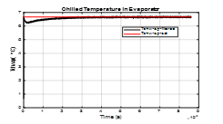Figure 16. Tchwsp – Moving Average filtered measurement noise impact on the MIMO control system response (noise level variance increased to 0.001, windows length = 10)

Figure 17. Refrigerant liquid level – Moving Average filtered measurement noise impact on the MIMO control system response (noise level variance increased to 1, window length =100 samples)

4.3. Closed-loop PI Control Strategies using Linear ARMAX SISO Models for Centrifugal Chiller System

In this section we develop two linear Auto Regressive Moving Average (ARMAX) SISO models for the both subsystems (Evaporator and Condenser) of the centrifugal chiller system (CCS). These two linear ARMA models are useful in this section to build and implement two PI closed-loop control strategies, and furthermore an interesting approach of a new control design approach, namely a PIP control strategy developed in next subsection 4.3.  To estimate the models’ parameters are used two particular MTLAB functions from Identification Toolbox, more precisely armax and arx. First one, armax MATLAB function estimates the parameters of ARMAX MIMO or SISO polynomial discrete-time models using time-domain data [17]. The data set of input-output chiller system measurements are generated by open-loop simulations performed on the SIMULINK model of chiller system shown in Figure 4, Figure 5.

  The second one, arx  MATLAB function  estimates the parameters of two polynomials discrete-time models known as Autoregressive with an exogenous input (ARX) and a more simple polynomial Autoregressive without exogenous input (AR) that estimates the parameters of  the scalar time series, by means of the well-known least squares method the most used  in control systems identification and parameters estimation. The both MATLAB functions use a prediction-error method and specified polynomial orders. For each of these models pure transport delays of the signals flow in the feedback path from the measurement sensors to the controllers for each input/output pair are also specified in their ARAMAX and ARX structures [17]. In addition, in each ARMAX and ARX model structures noise channels are incorporated, hence the most general polynomial form of these discrete-time models is given by [18 – 21]:

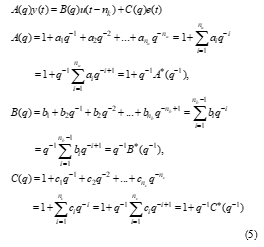where

• is the output at discrete-time t,  represent the degrees of the polynomials  and  respectively,
• is the control system input at the discrete instant t,
• is an integer number of sampling periods, the so-called dead time and most used in the control systems (pure transport delay of the signal flow between the measurement sensors and controllers in the feedback path,
• represent  the coefficients (parameters)  of the  polynomials and  of ARMAX models respectively,
• forward shift operator, i.e.  , and  backward shift operator, i.e. ,
• denotes  the normalized sampling time, only symbolic  that replaces the most used typical  notation   used to designate the description of dynamical discrete-time system,  representing the sampling period ,
• denotes the white noise disturbance value at the discrete instant t

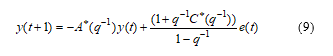
With these notations the general discrete-time representation of a dynamic system as ARMAX model can be put in the following form, as is given in [20]:

If the data are as  time series with no input channels and with only one output channel, then armax calculates an ARMA model for the time series, given by [1, 20]:

Furthermore, if in the noise source channel there is an integrator ARMAX model becomes an ARIMAX model, described by [19]:

If there are no inputs, the ARIMAX structure becomes an ARIMA model of the following form:

It is worth also to mention that the discrete-time representation in (6) can be put in a so called “regression form” useful to make the link with the least square estimation method of the ARMAX model coefficients and parameters based on the input-output data set measurements, as is mentioned in  [19]:

where the vectors  represent the vector of parameters:

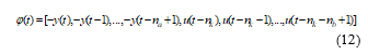
and the so called the “regressor vector” of measured values of the current outputs and the inputs and theirs the past values, respectively:

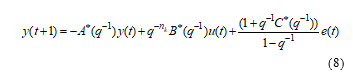
By means of some symbolic algebraic manipulations performed in the first equation (5) we get an interesting result that makes the link with the well-known discrete time “transfer operator” for open or closed loop control systems:

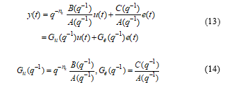where  and  represents the discrete time transfer operators for the channels input-output control system in open or closed-loop,  and “white” or “colored” noise channel – output control system,   respectively.

Moreover, if we replace formally in the equations (13) and (14) the shift (backward or forward) operator  by a complex variable  representing the real and imaginary parts of the complex variable s respectively, the most used by Laplace transform to compute the transfer functions of the control systems in the complex domain s,   a new representation in z complex domain is found, as follows:

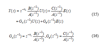This description is typically used for the control systems represented in discrete-time, where and are the z-images of the input , white noise , and the output , obtained by applying the  “transform Z” operator  to all three  discrete – time variables  , , and respectively [19]. The transfer operators , and defined in equation (16) are so-called z-transforms functions of the discrete-time control system.

In our case study, the discrete-time representations of the both SISO ARMAX models assigned to the centrifugal chiller control system are obtained in MATLAB R2017b by some manipulations of typical MATLAB functions in MATLAB code, given by [18-21]:

1. Chilled water temperature closed-loop SISO ARMAX discrete-time model:

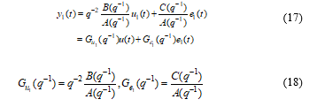and the polynomials are given by:

where the polynomials and have the orders 3, 3, and 6 respectively. The pure transport delay is samples, so the polynomials coefficients are given by:

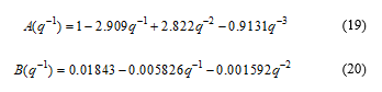
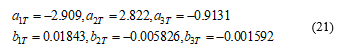1. Refrigerant liquid level closed-loop SISO ARMAX discrete-time model:

In Figure 18 we gather a valuable information about the validation of the both ARMAX models for entire range of the input-output measurements data set. To validate these two models in MATLAB can be used the typical MATLAB function called compare found in Identification MATLAB Toolbox. The input-output data set measurement of length 3006 samples are generated in open-loop simulations based on SIMULINK model of chiller system developed in section 3. The first segment of 1800 samples from input-output data set is used in prediction phase, and the second segment containing the samples between 1800 and 3006 is used in validation phase. The simulation results shown in Figure 18 reveal a very good estimation accuracy of the both ARMAX SISO models.

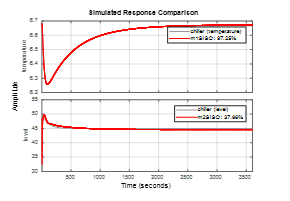Figure 18. Estimated ARMA SISO model validation for the booth closed-loops, chilled water temperature and Refrigerant liquid level

The closed-loop PI control laws for the both SISO ARMAX models are similar to those developed in the equations (1) – (4), but their design is more suitable in discrete-time to match the both SISO ARMAX models.  The both PI closed loops control strategies  are built in SIMULINK and the simulations results are performed partially in SIMULINK and finalized in MATLAB, as is shown in Figure 19, and Figure 20. In Figure 19 are shown the simulations results for chilled water temperature in Evaporator closed-loop control subsystem, and in Figure 20 can be seen the simulation results of  closed-loop PI controller performance for Refrigerant liquid level in Condenser subsystem. The both PI control loops are completely independent, without any interference between them. They are based on the decoupling loops assumption, proved in open-loop MATLAB simulation environment.  The simulation results reveal good accuracy and fast transient, especially for Refrigerant liquid level PI control shown in Figure 20. For the first approximate 500 samples the chilled water temperature in Evaporator reaches low values compared to measured temperature from  the input-output measurements data set required for the estimation, prediction and validation of both  ARMAX models. Fortunately, after this starting transient period the controlled chilled water temperature reaches the output measurements data set values with high accuracy.  This is an  interesting modelling key issue generated by  the  linearization of the plant dynamics, leading for a short period of time during the transient to a considerable degradation in PI controller performance. In addition the constraints on the operating range of the actuators could be also a big issue  for PI controller design. In contrast, the simulation results from Figure 20 reveal a very good accuracy, and also a fast transient.

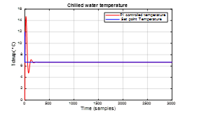Figure 19. PI controlled chilling water Evaporator temperature closed-loop ARMA SISO model compared to the set point temperature value

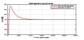Figure 20. PI controlled liquid level closed-loop ARMA SISO model compared

Set point level value

The Simulink models for the both PI controllers based on ARMAX SISO models are shown in Figure 21 and Figure 22, and also for more clearness they are attached in Annex-2. The rejection disturbance performance of both PI controllers is shown in Figure 23 and Figure 24.

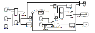Figure 21. The SIMULINK model of chilled water temperature PI closed-loop Evaporator control subsystem

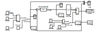Figure 22. The SIMULINK model of the Refrigerant liquid level PI closed-loop Condenser control subsystem

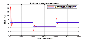Figure 23. Robustness of PI controlled chilling water Evaporator temperature closed-loop ARMA SISO model to the changes in set point temperature values

The simulations results in Figure 23 and Figure 24 show a great load disturbance rejection performance for both PI controllers. In fact, these results prove also the robustness of the both PI controllers for changes in the chiller system load.

Concluding, compared to the both PI control strategies developed in subsection 4.1, the proposed PI controllers in this subsection perform successful when using linear ARMAX SISO models for both control subsystems Evaporator and Condenser.

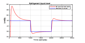Figure 24 Robustness of PI controlled refrigerant liquid level in Condenser closed-loop ARMA SISO model to the changes in set point level values

4.4. PPI Closed-Loop Controller Design using Linear ARMAX Models for Centrifugal Chiller Control System with Time Delay

The novelty of this subsection is a new design approach of the standard PI control strategy as a predictive discrete-time PI-plus (PIP) controller within the context of non-minimum state space (NMSS) control system, as is formulated in [13]. Furthermore, the non-minimal state space (NMSS) representation in contrast to minimal state space realizations “seems to be the natural description of a discrete-time transfer function, since its dimension is dictated by the complete structure of the model” as is stated in [13]. The minimal state space descriptions account only for the order of the denominator of the transfer function, and also the state variables assigned to each description not always  have physical meaning,  usually representing combinations of input and output signals [13]. Therefore, the resulting control algorithm in the new PIP control design approach within the NMSS context “can be interpreted as a logical extension of the conventional PI controller, facilitating its straightforward implementation using a standard hardware-software arrangement”, as is stated also in [13]. Further, the controller design methodology is the same as for an equivalent discrete-time Smith predictor (SP) controller for time delay systems, under certain non-restrictive pole assignment conditions, as is mentioned in [13].

The proposed PPI controller design follows the same methodology described in [13], encouraged by its great results obtained when applied in a MIMO ALSTOM nonlinear gasifier control plant [15]. Compared to the well-known Smith Predictor controller, in the new design approach the  predictive PI-plus controller  (PIPC) has more design flexibility and robustness [13].

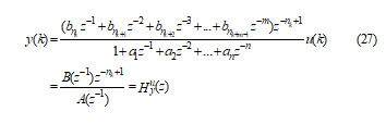
 Furthermore, the tuning parameters optimal selection, such as the weighting matrices required in the optimal performance criterion formulation can achieve multiple objectives. In addition, this new approach can be easy extended to MIMO PIPCs based on ARMAX models, such in [15]. In our case study the centrifugal chiller control system is represented in discrete-time by two SISO loops ARMAX models, given by the equations (17) – (21), and also in z-domain described by the equations (15) –(16). To simplify further the description in z-domain we neglect the white noise term, and the equations (15) and16) can be written in the following compact form, similar to those introduced in [13]:

In (27) represents the transfer function in z-domain of the output y of centrifugal chiller control SISO loop system with respect to corresponding control input u. Following the design control methodology described in [14], the model of the control system defined by the discrete transfer function given in (27) can be represented by the following NMSS equations:

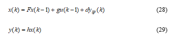where the  dimensional NMSS state vector  is defined as follows:

The new variable  introduced in (30) represents the discrete-time integral of error between the set point input (reference) and the control system output :

          The matrix F, and the vectors  are calculated based on the methodology described in [13-17]. Due to the editing constraints we give below only the matrix F and the vectors for a delay  since  matches the SISO temperature loop, and if is the case, for you can see the general description used in [13] for SISO systems, that can be also  extended for MIMO systems. Similar, in [15] is investigated the case    for a MIMO system that can be tailored on the Refrigerant liquid level SISO loop in our case study. For SISO systems with a delay  that matches also the temperature SISO loop, the matrix F and the vectors can be written as following [13]:

The element   of the vector  occupies the same position as the component occupies in the state vector  defined by (30). The components of the vectors  are identified straightforward due to their simple structures. A MIMO control system characterized by a transport delay  is described in [15] by the following expressions:

The control law related to the NMSS realization (28-30) takes the following state variable feedback (SVF) form [14-16]:

where the last component  of is the integrator gain of the first block located in the forward path of the PIP control diagram shown in Figure 25.

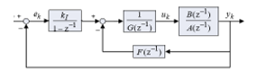Figure 25. PIP control block diagram (see [16])

It is worth to mention that the linear SVF control law (33) is easy to be implemented in practice, due to the facility storage of the variables in the MATLAB workspace. Furthermore, the inherent SVF formulation allows to investigate any SVF design methodology, such as:

• Poles assignment
• Linear quadratic (LQ) optimization
• Linear Quadratic Gaussian optimization
• optimization
• Linear exponential of quadratic Gaussian (LEQG) optimization

The poles assignment PIP controller design methodology in many cases is much simpler and intuitive, since the algebraic results are more perceptibly. In this paper we are focused only on the second approach, linear quadratic (LQ) optimization, but for the interested readers we try to provide only the steps of the poles assignment PIP controller design methodology, as follows:

Step1. Define a characteristic polynomial for the desired behavior of closed-loop PIP control system, i.e. choose the roots of the desired characteristic polynomial inside of unit circle  to assure the stability of the PIP control system in closed-loop, and to reach the desired performance (poles assignment).

The desired characteristic polynomial that meet the requirements from first step can be written as follows:

Step2. Compute the discrete time transfer function in closed-loop for the PIP control system that has the block diagram presented in Figure 24, as is given in [13]:

Step 3. Identify the polynomials coefficients  ,  of , and respectively, as well as the integrator gain :

Identification of the polynomials coefficients is based on the following poles assignment equation:

assuming that the closed-loop desired poles are located inside the unit circle to assure the stability, a good transient, as well as a good set point tracking.

The LQ optimization design approach is applied to the both closed-loops SISO ARMAX models (19-20), (25-26), considered as a starting point in order to design two PIP control laws.

Typically, the optimization criterion of LQ optimization design is defined in the same manner as for any quadratic optimization form written for a SISO control system:

where Q is a diagonal weighting matrix of the form:

and    is a positive scalar weight on the scalar input .

The resulting SVF gains are then obtained recursively from the steady state solution of the Algebraic Riccati Equation (ARE), derived from the standard LQ cost function (14) as follows [16]:

where the matrix P is a symmetrical positive definite matrix with its initial value , and  is the control gain vector for SVF.

1. PIP control law for chilled water  temperature closed-loop SISO ARMAX discrete-time Evaporator model described by:

The state associated to the PPI controller is given by:

and the PIP controller parameters computed according to (32) and (33) are given by:

The tuning parameters are set to:

The simulation results are shown in Figure 26  that reveal a very good tracking performance, fast transient, no oscillations, and a very small overshoot, perhaps the best performance obtained until now compared to previous temperature controllers.

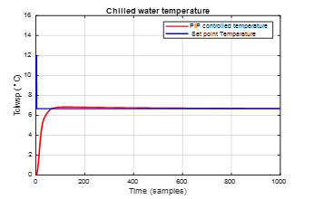Figure 26. PIP controlled chilling water Evaporator temperature closed-loop ARMA SISO model compared to the set point temperature value

1. PIP control law for closed-loop Refrigerant liquid level SISO ARMAX discrete-time  Condenser model described by:
2. The polynomials degree is smaller compare to temperature loop description, i.e. , thus the state vector will be of small dimension that simplify very much the PIP controller design, such as:

and the model parameters are calculated according to (34) replacing to match to an ARMAX SISO closed-loop control, as follows:

and the tuning parameters are set to

The Simulink models of PIP controllers are shown in Figure 27 for chilled water temperature control in Evaporator subsystem, and Figure 28 for liquid Refrigerant level control in Condenser subsystem, respectively.

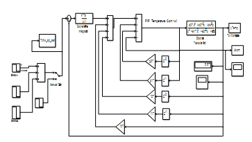Figure 27. The PIP controller of chilled water temperature in Evaporator Subsystem

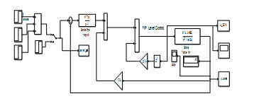Figure 28. The PIP controller of the liquid Refrigerant level in Condenser Subsystem

The simulation results are shown in Figure 29 that reveal a very fast transient and no oscillations, thus no overshoot and the overall behavior of PIP controller is as an aperiodic element. The same conclusion we can formulate that is the best performance obtained until now compared to previous Refrigerant liquid level controllers. Furthermore, we test the both PIP controllers for robustness to changes in set points, and the results reveal an excellent tracking performance for both, as is shown in Figure 30, and Figure 31 respectively.

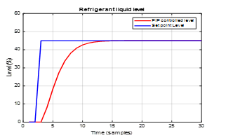Figure 29. PIP controlled Refrigerant liquid level closed-loop ARMA SISO model compared to the set point level value

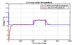Figure 30.The robustness to changes in input set point for closed-loop PIP controlled chilled water temperature in Evaporator subsystem described by an ARMA SISO model

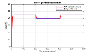Figure 31. The robustness to changes in input point set for closed-loop PIP controlled Refrigerant liquid level in Condenser subsystem described by an ARMA SISO model

Conflict of Interest

The authors declare no conflict of interest.

Conclusions

In our research work we introduce a new approach controller design, the so called in the literature as PI controller plus [13-16], definitely a new version of PI controller, but much simpler for design, and no more tuning parameters are required compared to standard version of PI controller, i.e. the coefficients . The third control strategy is an improved PI control version conceived within the context of non-minimum state space control systems with time delay.

 The non-minimal state space representation in contrast to minimal state space realizations “seems to be the natural description of a discrete-time transfer function, since its dimension is dictated by the complete structure of the model”, as is stated in [13]. Also, overall the new PIP controller developed in subsection 4.3 outperforms the first two PI controller’s versions proposed in the subsection 4.1 and 4.2 in terms of tracking performance, robustness, convergence speed and overshoot. Furthermore, the PIP controller can be easily extended to control MIMO systems with delay, as is done in [15], thus remains an open research topic for further investigations in the future work.

1. S. Bendapudi, J. E. Braun, et al., “Dynamic Model of a Centrifugal Chiller System – Model Development, Numerical Study, and Validation”, ASHRAE Trans., vol. 111, pp.132-148, 2005.
2. Beyene, H. Guven, et al., (1994),” Conventional Chiller Performances Simulation and Field Data”, International Journal of Energy Research, vol.18, pp.391-399, 1994.
3. J. E. Braun, J. W. Mitchell, et al., “Models for Variable-Speed Centrifugal Chillers”, ASHRAE Trans. , New York, NY, USA, 1987.
4. M. W. Browne, P. K. Bansal, “Steady-State Model of Centrifugal Liquid Chillers”, International Journal of Refrigeration, vol. 21, no.5, pp. 343-358, 1998.
5. B.E. Deepa Th. Mannath, “Study and Simulation of the Predictive Proportional Integral Controller in comparison with Proportional Integral Derivative controllers for a two-zone heater system”, Master Thesis, Texas Tech University, 2002.
6. M. Dhar, W. Soedel, “Transient Analysis of a Vapor Compression Refrigeration System”, in The XV International Congress of Refrigeration, Venice, 1979.
7. J.M. Gordon, K. C. Ng, H.T. Chua, “Centrifugal chillers: thermodynamic modeling and a diagnostic case study”, International Journal of Refrigeration, vol.18, no. 4, pp.253-257, 1995.
8. Li Pengfei, Li Yaoyu, J. E. Seem, “Modelica Based Dynamic Modeling of Water-Cooled Centrifugal Chillers”, International Refrigeration and Air Conditioning Conference, Purdue University, pp.1-8, 2010. http://docs.lib.purdue.edu/iracc/1091.
9. P. Popovic, H. N. Shapiro, “Modeling Study of a Centrifugal Compressor”, ASHRAE Trans., Toronto, 1998.
10. M. C. Svensson, “Non-Steady-State Modeling of a Water-to-Water Heat Pump Unit”, in Proceedings of 20th International Congress of Refrigeration, Sydney, 1999.
11. H. Wang, S. Wang, “A Mechanistic Model of a Centrifugal Chiller to Study HVAC Dynamics”, in Building Services Engineering Research and Technology, vol. 21, no.2, pp. 73-83, 2000.
12. A, Nada, E. M. Shaban, “The Development of Proportional-Integral-Plus Control Using Field Programmable Gate Array Technology Applied to Mechatronics System”, American Journal of Research Communication, vol. 2, no.4, pp.14-27, 2014.
13. C J Taylor, A Chotai and P C Young, “Proportional-integral-plus (PIP) control of time delay systems”, in Proceedings of the Institute Mechanical of Engineers, vol. 212, no.1, pp.37-47, 1998.
14. P. C. Young, A. P. McCabe, A. Chotai “State-dependent parameter nonlinear systems: Identification, Estimation and Control”, in IFAC, 15th Triennial World Congress, Barcelona, Spain, 2002.
15. J. Taylor and E.M. Shaban, “Multivariable Proportional-Integral-Plus (PIP) control of the ALSTOM nonlinear gasifier simulation”, in IEE Proceedings Control Theory and Applications, vol. 153, no.3, pp.277–285, 2006.
16. E. M. Shaban, A. A. Nada, “Proportional Integral Derivative versus Proportional Integral plus Control Applied to Mobile Robotic System”, Journal of American Science, vol.9, no.12, pp.583-591, 2013, doi:10.7537/marsjas091213.76.
17. M. Zaheeruddin, N. Tudoroiu, “Neuro – PID tracking control of a discharge air temperature system”, Elsevier, Energy Conversion and Management, vol. 45, pp.2405–2415, 2004.
18. MATLAB R2017b Documentation, https://www.mathworks.com/help/ident/ref/armax.html. Accessed at February 3rd, 2018.
19. I.D. Landau, R. Lozano, M. M’SAAD, A. Karimi, Adaptive Control – Chapter 2: Discrete-Time System Models for Control, Springer Link, pp. 35-53, 2011, DOI: 10.1007/978-0-85729-664-1_2.
20. L. Ang, “Comparison between Model Predictive Control and PID Control for water-level maintenance in a two-tank system”, Master Thesis, University of Pittsburgh, 2010.
21. Carnegie Mellon Lab, University of Michigan, “Control Tutorials for MATLAB”, http://ctms.engin.umich.edu.
22. M. Ning, “Neural Network Based Optimal Control of HVAC&R Systems”, PHD Thesis, Department of Building, Civil and Environmental Engineering. Montreal, Quebec: Concordia University, 2008.
23. ASHRAE Handbook-HVAC Systems and Equipment, 2008.
24. S.A. Korpela, Principles of turbomachinery. A John Wiley & Sons, Inc., Publication. 2011.
25. S.P.W. Wong and S.K. Wang,” System Simulation of the performance of a Centrifugal chiller Using a Shell-and-Tube-Type Water-Cooled Condenser and R-11 as Refrigerant”, in ASHRAE Trans, pp.445-454, 1989.
26. F.W. Yu and K. T. Chan, “Improved Condenser Design and Condenser-Fan Operation for Air-Cooled Chillers”, Applied Energy vol. 83, pp. 628-648, 2006.

(Click Here)

(Click Here)