1. Introduction

Intensive research interests have been in adaptive transmission techniques over wireless channels to efficiently support multimedia services, Internet access, 4G and future 5G mobile communications. One important issue is the ability to combat inter-symbol interference (ISI) in the wideband transmission over multipath fading channels.

Multicarrier modulation technique, such as orthogonal frequency division multiplex (OFDM), appears to be a promising solution to this problem. It is expended in various broadcast technologies like wireless local area network (WLAN), worldwide interoperability for microwave access (WiMAX), long term evolution (LTE), digital video broadcasting (DVB) and digital audio broadcasting (DAB) [1]. OFDM is a multicarrier system which employs a prominent number of close spaced carriers that are regulated with low data rate. In order to avoid mutual interference, the signals are made as orthogonal to each other. Coded Orthogonal Frequency Division Modulation (COFDM) is a kind of OFDM where error correction coding is comprised into the signal [2]. This system is able to attain excellent performance on frequency selective channels because the merged benefits of multicarrier modulation and coding. The multicarrier transmission reaches better results if incorporated with additive techniques in order to achieve higher efficiency in terms of throughput and ASE. The AMC-COFDM systems allows to choose the most appropriate Modulation and Coding Scheme (MCS) depending on the quality of the received signal and the channel conditions.

The aim of this paper is to develop an adaptive technique that improve the COFDM system performances: keep the error probability below a specified threshold or maximize the ASE. The MCS selection is based on the amount of received packets with errors, having as target that of minimizing that number and reducing the implementation complexity by using NLMS algorithm.

The rest of this paper is organized as follows. Section 2 gives the COFDM description where we show how the COFDM is better than OFDM.  In Section 3, we present the details of AMC system and explain NLMS algorithm for channel estimation. Simulation results have been discussed in Section 4 and finally, conclusions are provided in the last section.

2. COFDM System Description

The Coded Orthogonal Frequency Division Multiplexing (COFDM) system comprises of three main elements. These are Guard interval/cyclic prefix (CP), Channel coding/interleaving and IFFT. These technical aspects make the system tolerant to multipath fading and ISI [3]. Description of this transceiver system is listed:

The digital bits are randomly generated, convolutional coding is applied with different coding rate schemes (R=1/2, 2/3 or 3/4). The coded data is then interleaved to eliminate the effect of selective fading. The data is thereafter modulated using different proposed schemes (M-PSK, M-QAM). A serial-to-parallel conversion is performed. Thereafter, an IFFT is executed and guard time is added prior to parallel-to-serial conversion for making OFDM symbols tolerant to ISI. The data is thereafter digital-to-analog converted (DAC) and transmitted over the Rayleigh fading channel. At the receiver level, time and frequency synchronization is performed. The GI is removed and serial-to-parallel conversion is performed, and then an FFT is executed. The channel is estimated for each sub-carrier and the channel frequency selectivity is compensated for (equalized). After a final parallel-to-serial conversion, the data can then be demodulated and decoded. In order to achieve better performance, the receiver has to know the channel effect.

3.  AMC-COFDM Proposed System

Figure 1 illustrates the block scheme of structure of the proposed AMC-COFDM system, exploiting her potentialities taking that the change of modulation level and coding rate according to the CSI, for each symbol. The block diagram represents the whole system model. Basically, the proposed system is divided in two main sections namely transmitter and receiver:

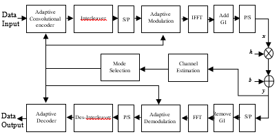Figure 1. The proposed AMC-COFDM transceiver block diagram.

At the transmitter level, the digital bits are randomly generated and encoded using an adaptive conventional coding technique, where three coding rates are proposed (1/2, 3/4, 2/3) with a constraint length of 3 and a polynomial generator [7,5]8. The sequence at the encoder output is permuted. The employed interleaver should have the capability of breaking up low-weight input sequences so that the permuted sequences have large distances between the 1’s.  Thus the incoming serial coded sequence is divided into low-rate data streams that are simultaneously transmitted, where each of the low-rate data streams is mapped using an adaptive modulation technique. There are four available modulation types for modeling the data onto sub-carriers: BPSK, QPSK, 16-QAM and 64-QAM used with gray coding in the constellation map. Depending on the feedback information, from the receiver, the mapping scheme and coding rate are adjusted.

The next stage consists to perform invers fast Fourier transform (IFFT), insert a guard area (GI) by the addition of cyclic prefix (CP). thus combating the inter-symbol interference (ISI) and inter-carrier interference (ICI) introduced by the multipath fading channel. As a last step Before the transmission through channel, a parallel to serial conversion is made.

As shown in the diagram block, at the reception level the inverse procedure is performed, where the serial to parallel conversion, the CP remove, and FFT are executed. To obtain the original data bits, the reverse process (demapping, de-interleaving, Viterbi decoding) is executed.

Besides, the NLMS channel estimator method is used. The knowledge on the Channel Impulse Response (CIR) provided by this method to the detector, is transmitted also through feedback channel. The basic concept of this channel estimation algorithm is to know sequence of bits, which is reoccurred in every transmission burst. The transferred symbols going through the channel transmission, can be regarded as a circular convolution between the CIR and the transmitted data block. In the receiver side, the channel coefficients are normally unknown. It demands to be efficiently estimated to maintain a low computational complexity.

3.1.  Least Mean Square (LMS) Algorithm

The Least Mean Square (LMS) algorithm was first developed in 1959 by Widrow and Hoff through their studies of pattern recognition [4]. From then it became one of the most widely used algorithms in adaptive filtering. The LMS is an adaptive filter algorithm known as stochastic gradient-based algorithm since it utilizes the gradient vector of the filter tap weights to converge on the optimal wiener solution [5,6]. It is well known by his computational simplicity and implementation facility. This simplicity that made it the benchmark against which all other adaptive filtering algorithms are judged. With each iteration of our algorithm, the tap weights of the adaptive filter are updated according to the following relation:

Where  represents the input vector of time delayed input values:

The vector is the coefficients of adaptive FIR filter tap weight vector at time  . The parameter µ is step size (a small positive constant) which controls the influence of the updating factor. The choice of a suitable value for μ is imperative to the performance of the LMS algorithm, if it is too small the time the adaptive filter takes to converge on the optimal solution will be too long; if μ is too large the adaptive filter becomes unstable and its output diverges [7,8].

The three distinct steps required for each LMS algorithm iteration are given as follows:

• First, the output of the FIR filter is calculated by following equation:

• Then, we calculate the error estimation value using the following relation:

• Thereafter, the tap weights of the FIR vector are updated using the relation (1) in preparation for the next iteration.

The primary trouble of the LMS algorithm is its sensitivity to the scaling of its input signals. This causes it very hard to select h that guarantees stability of the algorithm. Also, among its disadvantages is having a fixed step size parameter for every iteration [9]. This requires an understanding of the statistics of the input signal prior to commencing the adaptive filtering operation. In practice this is rarely achievable.

3.2.  Normalized Least Mean Square (NLMS)Algorithm

The normalized least mean square algorithm (NLMS) is a variant of the LMS algorithm that resolves these problems by annealing with the power of the input signal and calculating maximum step size value, it is proportional to the inverse of the total expected energy of the instantaneous values of the coefficients of the input vector . [i.e. Step size=1/dot product (input vector, input vector)].

The recursion formula for the NLMS algorithm is given by the following equation:

• Implementation of the NLMS algorithm:

We implement the NLMS algorithm in MatLab. It gives a great stability with unknown signals since the step size parameter is selected based on the current input values. The NLMS algorithm practical implementation is similar to that of the LMS algorithm. Each iteration of this algorithm requires these following steps:

first, we calculate the output of the adaptive filter using the following relation:

Then, we calculate the error estimation value using the relation (4).

Thereafter, the step size value for the input vector is determined by:

And then, the filter tap weights are updated using the relation (5) [i.e.

] in preparation for the next iteration.

3.3.  Analysis of Simulated Algorithms

In this section, we will examine the performance of LMS algorithm in comparison with the NLMS algorithm. The adaptive filter is a 1025th order FIR filter. The step size was set to 0.0005.

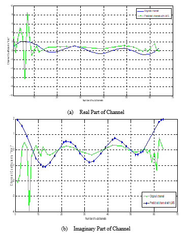Figure 2. Channel estimation using the LMS algorithm.

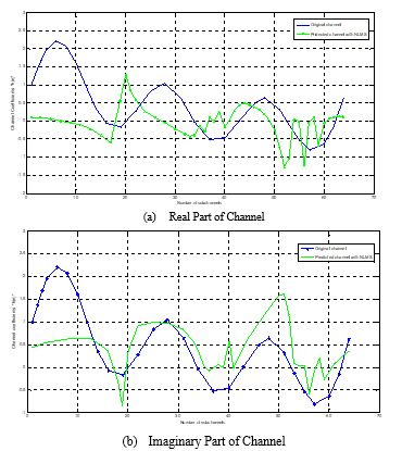Figure 3. Channel estimation using the NLMS algorithm.

Figure 2 shows the original and predicted values of channel coefficients with LMS algorithm, but the tracking is not efficient. It does not predict the coefficients exactly. So, NLMS algorithm is adopted to have better tracking compared to LMS. It is shown in figure 3.

The LMS algorithm is the most popular adaptive algorithm because of its simplicity. However, the LMS algorithm suffers from slow and data dependent convergence behavior. The NLMS algorithm, an equally simple, but more robust variant of the LMS algorithm, exhibits a better balance between simplicity and performance than the LMS algorithm. Due to its good properties the NLMS has been largely used in real-time applications.

4. Simulation Results

This paper considers a NLMS-AMC-COFDM binary transmission system. The Simulation model was implemented in MatLab. The system parameters used in simulations are given in Table 1.

Table 1. Parameters definition.

Parameter	Values
Number of sub channels	1024
Number of pilots	128
GI	256
Number of subcarriers	896
Channel length	16
Modulation schemes	BPSK, QPSK, 16QAM, 64QAM

In this section throughput vs. SNR performance is compared for various combination “modulation – code rate” schemes (BPSK1/2, QPSK 3/4, 16QAM 3/4 and 64QAM 2/3) with NLMS-Coded OFDM. In adaptive modulation and coding (AMC) technique modulation scheme and convolution code rate are altered according to the variation in the communication channel. The transmitter will choose the appropriate combination scheme is depend upon the SNR threshold.

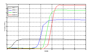Figure 4. Throughput of AMC schemes for NLMS-COFDM system.

Figure 4 presents the throughput versus SNR graphs for different proposed combination schemes selected by channel estimator using the COFDM scenario. We observe that 64QAM with code rate 2/3 offers a significant performance gain of 3dB to 4dB. As we see here, at a given SNR NLMS-COFDM can provide a significant increase in throughput when combined with suitable link adaptation, since higher throughput modes can be used at much lower values of SNR.

AMC increases the robustness of the system. In this way, the spectral efficiency of NLMS-COFDM and NLMS-AMC -COFDM are exploited in figure 5 to improve the performance. At lower SNR values BPSK is preferred because it gives lower BER values compared to remaining techniques. As modulation order increases, SE also increases for a given SNR value.

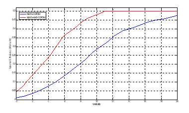Figure 5. Spectral Efficiency of AMC-NLMS-COFDM.

5. Conclusion

This paper exploits the Coded OFDM performance in terms of SE and throughput for different modulation and code rate schemes over a fading channel. COFDM is powerful modulation technique to achieve higher bit rate and to eliminate ISI. So, the COFDM has chosen for high speed digital communications of the next generation. This paper discusses the importance of Adaptive Modulation Coding technique. NLMS channel estimator is considered because of its low complexity. The most suitable MCS is chosen at the transmitter on the basis of channel estimator in terms of BER.

1. K. Chronopoulos, G. Tatsis, V. Raptis and P. Kosta- rakis, “Enhanced PAPR in OFDM without Deteriorating BER Performance” International Journal of Communications, Network and System Sciences, 4 (3), 164-169, 2011. https://doi.org/10.4236/ijcns.2011.43020
2. Chen, H.M. and Chen, W.C. and Chung, C.D. “Spectrally precoded OFDM and OFDMA with cyclic pre x and unconstrained guard ratios”, Wireless Commun., IEEE Trans., 10(5), 416-1427, 2011. https://doi.org/1109/TWC.2010.041211.091801
3. Fantacci, R. and Marabissi, D. and Tarchi, D. and Habib, I., “Adaptive modulation and coding techniques for OFDMA systems”, Wireless Commun., IEEE Trans., 8(9), 4876-4883, 2009. https://doi.org/1109/TWC.2009.090253
4. Soria, E.; Calpe, J.; Chambers, J.; Martinez, M.; Camps, G.; Guerrero, J.D.M.; “A novel approach to introducing adaptive filters based on the LMS algorithm and its variants”, IEEE Trans., 47(1), 127-133, Feb 2008. https://doi.org/1109/TE.2003.822632
5. N ; Pradeep. K ; Poonam. B;” An approach to implement LMS and NLMS adaptive noise cancellation algorithm in frequency domain”, IEEE Confluence The Next Generation Information Technology Summit (Confluence), Noida, India, 2014. https://doi.org/ 10.1109/CONFLUENCE.2014.6949268
6. Lee, K.A.; Gan,W.S; “Improving convergence of the NLMS algorithm using constrained subband updates”, Sig. Proc. Let. IEEE, 11(9), 736-739, 2004. https://doi.org/1109/LSP.2004.833445
7. G. Soumya ; N. Naveen ; M. J. Lal ; ”Application of Adaptive Filter Using Adaptive Line Enhancer Techniques”, IEEE Advances in Computing and Communications (ICACC), Cochin, India, 2013. https://doi.org/10.1109/ICACC.2013.39
8. L ; Xiaoli Xi ; “A New Variable Step-Size NLMS Adaptive Filtering Algorithm”, IEEE Information Technology and Applications (ITA), Chengdu, China, 2014. https://doi.org/10.1109/ITA.2013.62
9. Sajjad A. G.; Muhammad F. S.;” System identification using LMS, NLMS and RLS”, IEEE Research and Development (SCOReD), Putrajaya, Malaysia, 2013. https://doi.org/1109/SCOReD.2013.7002542

(Click Here)

(Click Here)