1. Introduction

Designing and planning component deployment of a cloud-hosted application with multiple tenants demands special consideration of the exact category of components that are to be distributed, the number of components to be shared, and the supporting cloud resources required for component deployment. [1] This is because there are different or varying degrees of multitenancy isolation. For instance, in components providing critical functionality, the degree of isolation is higher compared to components that only require slight re-configuration prior to deployment [2].

A low degree of isolation actively encourages tenants to share resources and components, resulting in lower resource consumption and reduced operating costs, however, there are potential challenges in both security and performance in the instance where one component sees a sudden workload surge. A high degree of isolation tends to deliver less security interference, although there are challenges instigated by high running costs and resource consumption in view that these tenants are not sharing resources [2]. Consequently, the software architect’s main challenge is to first identify solutions to the opposing trade-off of high degrees of isolation  (including excessive resource consumption issues and high operating costs), versus low degrees of isolation (including performance interference issues).

Motivated by these key challenges,  this paper presents a model for the deployment of components which provides exemplary solutions specific to cloud-based applications and aims to do so in a way that secures the segregation of multitenancy. The approach for this research includes creating an optimization model which is mapped to a Multichoice Multidimensional Knapsack Problem (MMKP) before solutions are tested using a metaheuristic. The approach is analysed through comparing the different optimal solutions achieved which then collectively compose an exhaustive search tool to analyse the solutions capacity specifially for minor problem occurance, in its entireity.

This paper and its research questions: “How can we optimize the way components of a cloud-hosted service is deployed for guaranteeing multitenancy isolation?”. It is possible to guarantee the specific degree of isolation essential between tenants, whilst efficiently managing the supporting resources at the same time through component deployment optimization of the cloud-based application.

This paper expands on the previous work conducted in [3]. The core contributions of this article are:

1. Mathematical optimization model providing optimal component deployment solutions appropriate for cloud-based applications to guarantee multitenancy isolation.
2. Mathematical equations inspired by open multiclass queuing network models to determine the average request totals for granting component and resource access.
3. Variants of metaheuristic solutions to deliver optimization model resolutions attributed to simulated annealing.
4. Guidelines and recommendations for component deployment in cloud-hosted applications seeking to guarantee required levels of multitenancy isolation.
5. Application areas of a cloud-hosted service where it is possible for the optimization model to be directly applied to component deployment with the aim to guarantee required degree of multitenancy isolation.

The remainder of this paper is structured as outlined below: Section II focuses on the challenge of identifying and delivering near-optimal component deployment solutions specific to cloud-hosted applications that guarantee the essential levels of multitenancy isolation; Section III presents the Optimisation Model; the following section presents the Metaheuristic Solution;  Section V considers the Open Multiclass Queuing Model; Section VI evaluates the results and presents the experimental setup; Section VII discusses the results;  Section VIII discusses the model’s application areas for the model; and Section IX conclude with recommendations of future work.

2. Optimising the Deployment of Components of Cloud-hosted Application with Guarantee for Multitenancy Isolation

 This section examines multitenancy isolation, the conflicting trades-offs in delivering optimal deployment influenced by the varying degrees of multitenancy isolation, and other associated research on cloud resources and optimal allocation of such resources.

2.1. Multitenancy Isolation and Trade-offs for Achieving Varying Degrees of Isolation

In a multitenant architecture (also referred to as multitenancy), multiple tenants are able to access a single instance of a cloud service. These tenants have to be isolated when there are changes in workload.  In the same way that it is possible to isolate multiple tenants, it is also possible to isolate multiple components of a cloud-hosted application.

In this paper, we define “Multitenancy Isolation” as a way of ensuring that other tenants are not affected by the required performance, stored data volume, and access privileges of one of the tenants. accessing the cloud-hosted application [3] [4].

A high degree of isolation is achieved when there is little or no impact on other tenants when a substantial increase in workload occurs for one of the tenants, and vice versa. The three cloud patterns that describe the varying degrees of multitenancy isolation are:

(i) Dedicated Component: tenants cannot share components; however, a component may be associated with one or more tenants or resources;

(ii) Tenant-isolated Component: tenants can share resources or components, and isolation of these is guaranteed; and

(iii) Shared Component: tenants can share resources or components, but these remain separate from other components.

If components required a high degree of isolation between them, then each tenant requires that each component is duplicated. This can be expensive and also lead to increased resource consumption. On the other hand, there could also be a need for a low degree of isolation which could, in contrast, reduce cost and resource consumption. However, any changes in workload levels that the application cannot cope with risk interference [4]. The question, therefore, is how optimal solutions can be identified to resolve trade-offs when conflicting alternatives arise.

2.2. Related Work on Optimal Deployment and Allocation of Cloud Resources

Research on optimal resource allocation in the cloud is quite significant, however, much fewer studies focus on optimal solutions in relation to component deployment across cloud-based applications in a way which guarantees the required degree of multitenancy isolation. Researchers in [5] and [6] aim to keep cloud architecture costs to a minimum by implementing a multitenant SaaS Model. Other authors [7] concentrated on bettering execution times for SaaS providers whilst reducing resource consumption using evolutionary algorithms opposed to traditional heuristics. A heuristic is defined in [8] for the capacity planning purposes for the SaaS inspired by a utility model. The aim of the utility model was to generate profit increases and so it largely concentrated on business-related aspects of delivering the SaaS application.

It is explained in [9] how optimal configuration can be identified for virtual servers, such as using certain tests to determine the required volumes of memory for application hosting. Optimal component distribution is discussed and analyzed by [10] in relation to virtual servers. Research conducted in [11] is of a similar nature to this paper in that it attempts to reduce costs (using a heuristic search approach is inspired on hill climbing), specifically in relation to the use of VMs from an IaaS provider with limitations around SLAs response time.

The studies noted above predominantly focus on scaling back costs associated with cloud architectural resources. The use of metaheuristics is not considered in these studies in delivering optimal solutions that can guarantee the required degree of multitenancy isolation. Additionally, previous research involving

optimization models have operated with one objective; an example is where [11] look to minimize VM operational costs. For this paper’s model, a bi-objective case is used (i.e., maximising the required degree of multitenancy isolation and number of requests permitted to access a component). Thereafter, a modern metaheuristic inspired by simulated annealing is used to solve the model.

3. Problem Formalization and Notation

This section defines the problem and explains the process of mapping it to a Multichroic Multidimensional Knapsack Problem (MMKP).

3.1. Description of the Problem

Assuming a tenant has multiple components associated with the same supporting cloud infrastructure. A team may represent a team or department, a company with a responsibility to design a cloud-based application, its components, and underlying processes. Components varying in size and function has to integrate with their cloud-hosted application to achieve effective deployment in a multitenant style. It is also possible to define component categories based on different features, such as function, for example, processing or storage. Within these categories, different components are likely to have differing degrees of isolation enabling some components to deliver the same function which can hence be accessed and used by multiple tenants, opposed to other components which may be solely allocated to certain tenants or departments.

Every component within an application needs a particular allocation of resources from the cloud infrastructure in order to support the volume of requests received. In instances where one component in the application experiences surges in workload, then it must be considered how the designer can choose components to deliver optimal deployment to effectively respond to the sudden changes in such a manner that: (i) maximises component degrees of isolation through ensuring they behave in the same way as components of other tenants, thus, isolating against one and other; and (ii) maximises the total requests permitted to access and use each components.

3.2 Mapping the Problem to a Multichoice Multidimensional Knapsack Problem (MMKP)

The above mentioned optimal component deployment problem can be closely linked to a 0-1 Multichoice Multidimensional Knapsack Problem (MMKP). An MMKP is a variant of the Knapsack Problem commonly depicted as a member of the NP-hard class of problems. For the purpose of this paper, the problem of focus can be formally defined as:

Definition 1 (Optimal Component Deployment Problem): Consider that there are N groups of components (C₁,…,C_N) with each group having a_i (1 ≤ i ≤ N) components useful for designing (or integrating with) a cloud-hosted application. Each component of the application is affiliated with: (i) the degree of isolation that is required between components (I_ij); (ii) the rate at which requests arrive to the component λ_ij; (iii) the service demand of resources required to support the component D_ij; (iii) the average request totals permitted to access the component Q_ij and (iv) resources for  supporting the component, r_ij = r_ij¹ ,r_ij² ,…,r_ijⁿ . For the cloud to properly support all components, a certain volume of resources are required; the total number of resources needed can be calculated as R = (R¹,R²,…,Rⁿ).

The aim of an MMKP is to choose one component present in each category for deployment to the cloud in a manner that ensures that if one component sees sudden increases in load, then the: (a) the degree of isolation of other components is maximized;         (b) the total requests permitted to access the component and application is maximised without using more resources than are actually available.

Definition 1 identifies two objectives within the problem. An aggregation function is used to convert the multi-objective problem into a single-objective because of merging the two objective functions merge (i.e., g1=degree of isolation, and g2=number of requests) into one single objective function (i.e., g=optimal function) in a linear way. Because the optimal function of this study is linear, a priori single weight strategy is employed to aid defining the weight vector selected based on the decision maker’s individual preferences [12]. This paper also adopts the approach discussed in [12] for computing the absolute percentage difference (see section 7.1), the target solutions used to compare against the optimal solution (see section 7.2), and the use of the number of optimal function evaluations as an alternative to measuring the computational effort of the metaheuristic.

Therefore, the purpose is redefined as follows: to deliver a near-optimal solution for component deployment to the cloud-based application that also fulfils system requirements and achieves the best value possible for optimal function, G.

Definition 2 (Optimal Function): For a cloud-hosted application architect, the main issues impacting the optimal deployment of components are changes to workload, which can be expressed as:

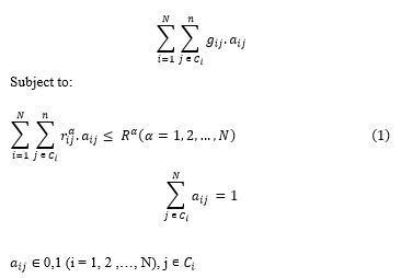
where (i) a_ij is fixed at 1 if component j is chosen from group C_i and 0 otherwise; (ii) g_ij is determined by a weighted calculation of parameters involving the degree of isolation, average requests permitted to access a component, and penalty for constraint violations.

Specific weight values are allocated to w1, w2, and w3; namely 100, 1 and 0.1 respectively. The allocation of weights is done using a method that provides preference to the required degree of isolation. The penalty, P_ij, imposed for components that surmount resource cap is expressed as: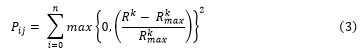

For every component (g), the degree of isolation, I_ij, is assigned either 1, 2, or 3 indicating either shared, tenant-isolated or dedicated components, respectively. The sum described as:  refers to the resource consumption in group C_i.  for each individual application component j. Total resource consumption  for all application components needs to be lower than the total available resources in the cloud infrastructure R = R^α,(α = 1,…,m).

It is presumed that the service demands at the CPU, RAM, Disk I/O, and the supporting bandwidth of each component can be identified and/or measured readily by the SaaS supplier or customer. This assumption enables us to calculate the number of requests, Q_ij that may be permitted access for each component through analysis of an open multiclass QN Model [13]. The following section expands further on the open multiclass network.

4. Queuing Network (QN) Model

Queueing network modelling is one modelling approach through which the computer system is depicted as a network of queues that can be solved in an analytic fashion. In its most basic form, a network of queues is an assembly of service centers representative of system resources, and customers representative of business activity, such as transactions [13]. Service centers are basically supporting resources for the components, such as CPU, RAM, disk and bandwidth.

Assumptions: For the purpose of this paper, the following component assumptions are made:

(i) components cannot support other applications or alternative system requirements, and is therefore exclusively deployed to one cloud-application;

(ii) component arrival rates are separate to the main system state and so component requests may have significantly varied behaviours.

(iii) it is possible to identify and effortlessly measure the service demands at the CPU, RAM, Disk, and Bandwidth supporting each component by both the SaaS provider and/or customer.

(iv) sufficient resource is available to support each component during changes to workload, particularly during significant surges of new incoming requests. Ensuring sufficient resource means that there are no overloads during peak times where all components are operating.

The assumptions noted above allow the study to utilise an open multiclass queuing network (QN) model for the purpose of calculating average requests permitted to reach the component, whilst simultaneously ensuring the required degree of isolation, as well as system requirements. The magnitude and intensity of workload volume in an open multiclass QN is determined by request arrival rates. The arrival rate is not typically reliant on the system state, and so is not reliant on the volume of other tenants in the system either [13].

Definition 3 (Open Multiclass Queuing Network Model): Assuming there is a total of N classes, where every class c is an open class with arrival rate λ_c. The arrival rates are symbolised as a vector by  = (λ₁, λ₂, … λ_N). The use of each component in class c at the center k is given by:

To solve the QN model, assumptions are made, such as that a component stands for a single open class system hosting four service centers otherwise referred to as supporting resources, such as CPU, RAM, disk capacity and bandwidth. At any one service center (e.g., CPU), the average request totals for a specific component is: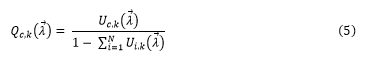

Consequently, to determine the average amount of requests accessing the particular component, the length of the queue of all requests reaching all service centers (i.e., components’ supporting resources such as CPU, RAM, disk capacity and bandwidth) would be totaled.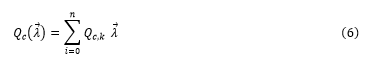

5. Metaheuristic Search

The optimisation problem as explained in the section before is an NP-hard problem renowned for its feasible search capacity and exponential growth [14]. The number of potential and feasible solutions that may achieve optimal component deployment and solve the problem can be determined using this equation:

The above equation, Equation 4, signifies the different ways one or more (r) components can be chosen from each group (comprising of n components) from a pool of numerous (N) groups of components, for the purpose of creating and integrating them into a cloud-hosted application upon receipt of updates or changes to workload by the component. Thus, to manage such changes to workloads, the specific number of different ways that one component can be selected (i.e., r=1) from each of the 20 different groups (i.e., N=20), comprising of 10 items per group (i.e., n=10), approximately 10.24 x 10¹² possible solutions can be identified. Contingent on the number of changes to workload and also the regularity of these, a cloud-hosted service quite large in size could experience a much greater volume of possible solutions.

Therefore, to obtain an optimal solution for the identified optimisation problem, it is essential to use an efficient metaheuristic. In addition, this should be done in real-time with the SaaS customer or cloud architect. Two versions of a simulated annealing algorithm are implied: (i) SAGreedy, incorporates greedy principles in conjunction with a simulated annealing algorithm; (ii) SARandom, employs randomly propagated solutions in conjunction with a simulated annealing algorithm. Both of these versions can be effectively utilised to achieve near-optimal solutions for component deployment. Additionally, an algorithm was developed for this study to generate an extensive search of the full solution area for a small problem size. Algorithm 1 includes the algorithm for SA(Greedy). However, SA(Random) only needs a minor change to this algorithm, which will be described further in the following section. An extensive breakdown of Algorithm 1 can be viewed below:

Algorithm 1 SA(Greedy) Algorithm
1:	SA (Greedy) (mmkpFile, N)
2:	Randomly generated N solutions
3:	Initial temperature fixed to T0 to st. dev. of all optimal solutions
4:	Create greedySoln a1 with optimal value g(a1)
5:	optimalSoln = g(a1)
6:	bestSoln = g(a1)
7:	for I = 1, N do
8:	Create neighbour soln a2 with optimal value g(a2)
9:	Mutate the soln a2 to improve it
10:	if a1 < a2 then
11:	bestSoln = a2
12:	else
13:	if random[0,1) < exp(-(g(a2) – g(a1))/T) then
14:	a2 = bestSoln
15:	end if
16:	end if
17:	Ti+1 = 0.9 * Ti
18:	end for
19:	optimalSoln = bestSoln
20:	Return (optimalSoln)

5.1. The SAGreedy for Near-optimal Solution

The first algorithm is a combination of simulation annealing and greedy algorithm which is used to obtain a near-optimal solution for the optimisation problem modelled as an MMKP. First, the algorithm extracts the key details from the MMKP problem instance before populating the encompassing variables (i.e., collections of different dimensions storing isolation values of isolation; average request totals; and the resource consumption of components). A basic linear cooling schedule is used, where T_i+1 = 0.9Ti. The method for prescribing and fixing the preliminary temperature T₀ will be to randomly generate an optimal solution whose number is equivalent to the total number of groups (n) in the problem instance, multiplied by the number of iterations (N) used in the experimental settings before running the simulated annealing element of the algorithm.

When the problem instance and/or the total iterations is low, the magnitude of optimal solutions created may be limited by the number of groups (n) in the problem instance, multiplied by total iterations (N) used in the experimental settings. Next, the initial temperature T₀ is determined for the standard deviation of all optimal solutions (Line 2-3) through random generation. The algorithm then uses the greedy solution as the preliminary solution (Line 4) which is assumed as the best current solution. The simulated annealing process enhances the greedy solution further providing a near-optimal solution for cloud component deployment.

The execution of the algorithm in its most basic form for the instance C(4,5,4) is explained as follows: let us imagine that the total number of iterations is 100, 400 (i.e., 4 groups x 100 iterations) optimal solutions are randomly generated before calculating the standard deviation for all solutions. Assuming a value of 50.56, T₀ is identified as 50. It is also assumed that the algorithm creates a foremost greedy solution with g(a¹) = 2940.12, before a current random solution with g(a²) = 2956.55. The solution a² will substitute a¹ with probability, P =exp(-16.43/50)=0.72, because g(a²) > g(a¹). In lines 14 to 16, a random number (rand) is generated between 0 and 1; if rand <0.72, a² replaces a¹ and we proceed with a². Alternatively, the study continues with a¹. Now, the temperature T is reduced providing T₁ = 45 (Line 17). Iterations continue until N (that is, the identified number of iterations set to enable the algorithm to function), is reached, thus the search converges with a high probability of near-optimal solution.

5.2. The SA(Random) for Optimal Solutions

Considering the SA(Random) metaheuristic version, a solution is also randomly generated before being encompassed within the simulated annealing process to provide a preliminary solution. It can be seen in Line 4 that rather than creating a greedy solution, a random solution is created. An optimal solution representative of a set of components with the highest total isolation value and number of requests permitted to reach the component access is then output by the algorithm. Every time a variance in workload is experiences, the optimal solution alters to respond to this.

6. Evaluation

We describe in the section how each instance was generated as well as the process, procedure and set up of the experiment.

6.1. Instance Generation

Reflective of different capacities and sizes, a number of problem instances were randomly generated. Instances were divided into two categories determined by those cited frequently in current literature: (i) OR benchmark Library [15] and other standard MMKP benchmarks, and (ii) the new irregular benchmarks used in [16]. All these benchmarks were used for single objective problems. This study edited and modified this benchmark to fit into a multi-objective case through assigning each component with one of two profit values: isolation values and average number of requests [17].

The values of the MMKP the instance, were produced as follows: (i) random generation of isolation values in the interval [1-3]; (ii) values of component consumption of CPU, RAM, disk and bandwidth (i.e., the weights) were generated in the interval [1-9]; (iii) individual component resource limits (i.e., knapsack capacities for CPU, RAM, disk and bandwidth) were created  by halving the maximum resource consumption possible (see Equation 7).

An identical principle has been employed to create instances for OR Benchmark Library, as well as for instances used in [18] [19]. This research considers the total resources/constraints as four (4) for each group, which reflects the minimal resource requirement to deploy a component to the cloud. The notation for each instance is: C(n,r,m), representing the number of groups, the amount of components in each group, and resource totals.

6.2. Experimental Setup and Procedure

For consistency, all experiments were set up and operated using Windows 8.1 on a SAMSUNG Laptop with an Intel(R) CORE(TM) i7-3630QM at 2.40GHZ, 8GB memory and 1TB swap space on the hard disk. Table I outlines the experimental parameters. The algorithm was tested using different sized instances of different densities. In relation to large instances, it was not possible to conduct an exhaustive search due to a lack of memory resource on the machine used.

As a result of this limitation, the MMKP instance was implemented first, C(4,5,4), to provide a benchmark for analysis to enable algorithm comparison.

Table 1. Parameters used in the Experiments

Parameters	Value
Isolation Value	[1,2,3]
No. of Requests	[0,10]
Resource consumption	[0,10]
No. of Iterations	N=100 (except Table 4)
No. of Random Changes	5
Temperature	T0 = st.dev of N randomly generated solns.
Linear Cooling Schedule	Ti+1 =0.9Ti

7. Results

Section 7 discusses the experiment results.

7.1 Comparison of the Obtained Solutions with the Optimal Solutions

The results delivered by algorithms SA(Greedy) and SA(Random) were initially compared with the optimal solutions generated by an exhaustive search for a small problem instance in the entire solution space (i.e., C(4,5,4)). Table 2 and Table 3 portray the findings. The instance id used is noted in Column 1 of Table 2. The second, third and fourth columns respectively highlight the optimal function variables as (FV/IV/RV), representing the optimal function value, isolation value, and number of permitted requests, for Optimal, SA(Random) and SA(Greedy) algorithms. The first and second columns of Table 3 depict a proportion of the optimal values for SA(Random) and SA(Greedy) algorithms, respectively. The final two columns note the absolute percentage difference, indicative of the solution quality, for SA(Random) and SA(Greedy) algorithms, which is measured as follows:

where s is the obtained solution and s* is the optimal solution generated by the exhaustive search.

It is clear that SA(Greedy) and SA(Random) provide very similar results. Solutions identified for SA(Random) are almost 100% close most of the time to their optimal solution, and over 83% in a smaller proportion of cases whilst in just one occurrence it was below 66%.  SA(Greedy) also delivered nearly 100% close solutions created to the optimal solution in a considerable number of cases, and more than 83% in others. Overall, SA(Greedy) delivered better results than SA(Random) when considering percent deviation from the optimal solution.

7.2 Comparison of the Obtained Solutions to a Target Solution

It was not possible to run instances greater than C(4,5,4) because of hardware limitations (i.e., CPU and RAM).

Consequently, the results were compared to a target solution. The target solution for percent deviation and performance rate was determined as (n x max(I) x w1) and ((n x max(I) x w1) + (0.5 x (n x max(Q) x w2))), respectively. So, for instance C(150,20,4), the target solution for computing percent deviation sit at 45,000.

Table III, IV, and V demonstrates average solution behaviour: (i) on a significant selection of varied instances using the same parameters; (ii) over various runs on the same instance (with differing quantities of optimal evaluation); and (iii) over different runs on the same instance. The robustness of solutions in relation to their behaviour on varying types of instances using the same parameters was measured. Table III shows this measure and that solutions are strong when considering average deviation of solution behaviour for both the SA(Greedy) and SA(Random), as implied through their low variability scores.

The average percent deviation and standard deviation (of the percent deviations), for SA(Greedy) is marginally greater than SA(Random) as a result of the significant absolute difference between some solutions and the reference solution. For example, the percent deviations of SA(Greedy) for the instances C(100,20,4) and C150,20,4) are higher than SA(Random). The results show how SA(Random) performs much better than SA(Greedy) in reference to small instances up to C(80,20,4).

Table IV compares solution quality with optimal function evaluations. It can be determined that the overall solution quality is good when both algorithms are tested on large instances. Once again, the standard deviation for SA(Greedy) is notably lower than SA(Random) in addition to great percent deviation stability. Table V highlighted that SA(Greedy) is stronger than SA(Random) evidenced by the average optimal values and low solution variability. The performance rate (PR) was computed by determining the reference solution as a function of the quantity of optimal evaluations. The PR of SA(Greedy) is marginally higher than SA(Random).

Figure I depict the relationship of solution quality relating to optimal values (i.e., fitness value) and the volume of optimal function evaluations. It can be seen from the diagram that SA(Greedy) benefited a little from the preliminary greedy solution more than SA(Random) when optimal function evaluations are few. Nonetheless, solution quality for both algorithms are better as iterations increase. Once 100 optimal evaluations are reached, the optimal solution stabilizes, but thereafter fails to show any further noticeable improvement.

Figure 2 portrays correlations between solution quality relating to percent deviation and the total function evaluations. In line with expectations, SA(Random) reported a smaller percent deviation than SA(Greedy) in the majority of results, particularly in instances where function evaluations are few. An explanation for this could be the low function evaluation total used in the study. However, percent deviation for SA(Greedy) showed greater stability despite being greater than SA(Greedy)’s results.

Table 2. Comparison of SA(Greedy) and SA(Random) with the Optimal Solution

Inst-id	Optimal (FV/IV/RV)	SA(R) (FV/IV/RV)	SA(Greedy) (FV/IV/RV)
I1	1213.93/12/24	1218/12/18	1218/12/18
I2	1213.97/12/14	1208.99/12/9	1109/11/9
I3	1222.99/12/23	1120/11/20	1120/11/20
I4	1119.98/11/20	1023/10/23	1019/10/19
I5	1219.99/12/20	1017/10/17	1017/10/17
I6	1229.92/12/30	1020.96/10/21	1022.99/10/23
I7	1224.90/12/25	1018/10/18	1018/10/18
I8	1228.96/12/29	822/8/22	1224.99/12/29
I9	1021.97/10/22	912/9/12	912/9/12
I10	1236/12/36	1236/12/36	1236/12/36

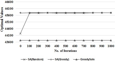Figure 1. Relationship between Optimal Values and Function Evaluations.

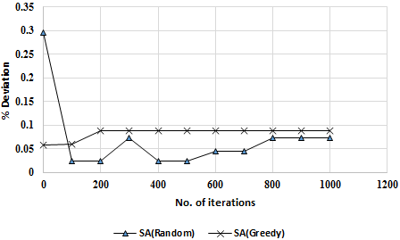Figure 2. Relationship between Percent Deviation and Function evaluations.

8. Discussion

In Section 8 the implication of the results is discussed further and recommendations for component deployment of a cloud-hosted application that guarantees multitenancy isolation are considered and presented.

8.1 Quality of the Solutions

Solution quality was measured encompassing percent deviation from either the optimal or reference solution. Tables II, III and IV note solutions generated by SA(Greedy) which demonstrate a low percent deviation. The results also indicate that SA(Greedy) performs efficiently for large instances. However, Table III clearly evidences SA(Random) outperforming SA(Greedy) on small instances, that is, from C(5,20,4) to C(80,20,4).

Table 3. Computation of a Fraction of the Obtained Solutions with the Optimal Solution.

Inst-id	SA-R/Opt		SA-G/Opt	%D (SA-R)	%D (SA-G)
I1	0.995		0.995	0.48	0.48
I2	0.996		0.914	0.41	8.65
I3	0.916		0.916	8.42	8.42
I4	0.913		0.910	8.66	9.02
I5	0.834		0.834	16.64	16.64
I6	0.830		0.832	16.99	16.82
I7	0.831		0.831	16.89	16.89
I8	0.669		0.997	33.11	0.32
I9	0.892		0.892	10.76	10.76
I10	1		1	0	0
ST.DEV	0.097		0.064	9.73	6.43

Table 4. Comparison of the Quality of Solution with Instance size

Inst (n=20)	SA-R	SA-G	SA-R	SA-G
C(5)	1528/15/28	1517/15/17	1.87	1.13
C(10)	3058/30/58	3057/30/57	1.93	1.9
C(20)	6082/60/82	6002/59/102	1.37	0.03
C(40)	12182/120/182	12182/120/182	1.52	1.52
C(60)	18317/180/317	18317/180/317	1.76	1.76
C(80)	24388/240/388	24380/240/380	1.62	1.58
C(100)	30252/298/452	30505/300/505	0.84	1.68
C(150)	45648/449/748	45793/450/793	1.44	1.76
Avg. %D			1.54	1.42
STD of Avg. %D			0.33	0.57

8.2. Computational Effort and Performance Rate of Solutions

Hardware limitations of the computer used for the study restricted evaluation and full consideration of computational effort for metaheuristics. On the other hand, it was still possible to compute algorithm performance rates as a function of optimal evaluation totals. Typically, the number of optimal evaluations is considered a computational effort indicator that is independent to the utilised computer system. Table V indicates that the performance rate of SA(Greedy) is marginally higher than SA(Random) when we put into consideration the total reference solutions achieved.

Table 5. Comparing Solution Quality vs. No. of Optimal Evaluations

No. of Iteration	SA(R)	SA(G)	%D (SA-R)	%D (SA-G)
1	44242.1	45776.8	3.30	0.06
100	45760.7	45776.9	0.02	0.06
200	45760.7	45790	0.02	0.09
300	45783	45790	0.07	0.09
400	45760.7	45790	0.02	0.09
500	45760.7	45790	0.02	0.09
600	45770.1	45790	0.04	0.09
700	45770.1	45790	0.04	0.09
800	45783	45790	0.07	0.09
900	45783	45790	0.07	0.09
1000	45783	45790	0.07	0.09
Worst	44242.1	45776.8	0.02	0.06
Best	45783	45790	3.30	0.09
Average	45632.46	45787.61	0.34	0.08
STD	439.77	5.07	0.93	0.01

8.3. Robustness of the Solutions

Low variability was seen from the SA(Greedy) algorithm particularly when run with large instances, therefore suggesting it delivers stronger solutions than SA(Random) making SA(Greedy) the most suitable algorithm for real-time use in a fast-paced environment experiencing regular changes to workload levels. Figure 1 demonstrates instability in SA(Random) for a small amount of evaluations, although following 1,000 evaluations it was seen to converge eventually at the optimal solution. In contrast, the SA(Greedy) showed steady improvement as evaluations increased.

8.4. Required Degree of Isolation

The study’s optimisation model assumes that each component for deployment (or group of components) is linked to certain degree of isolation. By mapping the problem to a Multichoice Multidimensional Knapsack Problem linking each component to a profit values: either isolation value; or number of requests permitted to access a component, this was achieved. As a result of this, it was possible to monitor each component separately and independently, responding to each of their unique demands. Where limitations are faced, such as through cost, time or effort used to tag each component, a different algorithm could enable us to perform this function dynamically. In our research prior to this [20], an algorithm capable of dynamically learning the properties of current components in a repository was developed with this information then used to associate each component with the required degree of isolation.

Table 6. Robustness of Solutions over Different Runs on the Same Instance.

Runs	SA(R)	SA(G)	%D SA-R	%D SA-G
1	45767	45658	1.70	1.46
2	45793	45744	1.76	1.65
3	45663	45793	1.47	1.76
4	45460	45658	1.02	1.46
5	45567	45658	1.26	1.46
6	45562	45793	1.25	1.76
7	45569	45658	1.26	1.46
8	45567	45658	1.26	1.46
9	45682	45658	1.52	1.46
10	45663	45767	1.47	1.70
Worst	45460	45658	1.02	1.46
Best	45793	45793	1.76	1.76
Avg	45629	45705	1.40	1.57
STD	97.67	58.40	0.22	0.13
Perf. Rate	2.0E-04	3.0E-04

 9. Application Areas for Utilizing the Optimization Model

In this section, we discuss the various areas where our optimization model can be applied to the deployment components of a cloud-hosted service for guaranteeing the required degree of multitenancy isolation.

9.1. Optimal Allocation in a resource constrained environment

Our optimization model can be used to optimize the allocation of resources especially in a resource constrained environment. or where there are frequent changes in workload. This can be achieved by integrating our model into a load balancer/manager. Many cloud providers have auto-scaling programs (e.g., Amazon Auto scaling) for scaling applications deployed on their cloud infrastructure, usually based on per-defined scaling rules. However, these scaling programs do not have a functionality to provide for guaranteeing the isolation of tenants (or components) associated with the deployed service. It is the responsibility of the customer to implement such a functionality for individual service deployed to the cloud. In an environment where there are frequent workload changes, there would be a high possibility of performance interference. In such a situation, our model can be used to select the optimal configuration for deploying a component that maximizes the number of request that can be allowed to access the component while at the same maximizing the degree of isolation between tenants (or components).

9.2. Monitoring Runtime Information of Components

Another area where our model can be very useful is in monitoring the runtime information of components. Many providers offer monitoring information on network availability and utilization of components deployed on their cloud infrastructure based on some pre-defined configuration rules. However, none of this information can assure that the component is functioning efficiently and guarantees the required degree of multitenancy isolation on the application level. It is the responsibility of the customer to extract and interpret these values, adjust the configuration, and thus provide optimal configuration that guarantees the required degree of multitenancy isolation.

Our model can be implemented in the form of a simple web service-based application to monitor the service and automatically change the rules, for example, based on previous experiences, user input, or once the average utilization of resources exceeds a defined threshold.  This application can be either be deployed separately or integrated into different cloud-hosted services for monitoring the health status of a cloud service.

9.3. Managing the Provisioning and Decommissioning of Components

The provisioning and decommissioning of components or functionality offered to customers by many cloud providers is through the configuration of pre-defined rules. For example, a rule can state that once an average utilization of a system resource (e.g., RAM, disk space) exceeds a defined threshold then a component shall be started. When runtime information of components is extracted, and made available as stated earlier, they can be used to make important decisions concerning the provisioning of required components and decommissioning of unused components.

10. Conclusion and Future Work

Within this research, to provide a further contribution to the current literature on multitenancy isolation and optimized component deployment, we have developed an optimisation model alongside a metaheuristic solution largely inspired by simulated annealing for the purpose of delivering near-optimal component deployment solutions specific to cloud-based applications that guarantee multitenancy isolation. First, an optimisation problem was formulated to capture the implementation of the required degree of isolation between components. Next, the problem was mapped against an MMKP to enable early resolution through the use of a metaheuristic.

Results show greater consistency and dependability from SA(Greedy), particularly when functioning on large instances, whereas SA(Random) operates sufficiently on small instances. When considering algorithm strength, SA(Greedy) portrayed low variability and thus generates higher quality solutions in dynamic environments experiencing regular changes in workload levels. SA(random) appears to have greater sensitivity and instability to small deviations of input instances compared to SA(Greedy), more so in relation to large instances.

We intend on testing the MMKP problem instances further using various metaheuristic types (e.g., genetic and estimated distribution algorithms) and combinations (e.g., simulated annealing merged with genetic algorithm) with the aim of identifying the most efficient metaheuristic to generate optimal solutions to operate in a variety of cloud deployment situations. For future research, a decision support system will be developed capable of creating or integrating an elastic load balancer for runtime information monitoring in relation to single specific components in order to deliver near-optimal component deployment solutions specific to responses required from cloud-hosted applications to changes in workload. This would be of immense value to cloud designers and SaaS customers for decision making around the provision and decommission of components.

Conflict of Interest

The authors declare no conflict of interest.

Acknowledgment

This research was supported by the Tertiary Education Trust Fund (TETFUND), Nigeria and IDEAS Research Institute, Robert Gordon University, UK.

1. Fehling, F. Leymann, R. Retter, W. Schupeck, and P. Arbitter, Cloud Computing Patterns. Springer, 2014.
2. Krebs, C. Momm, and S. Kounev, “Architectural concerns in multi-tenant saas applications.” CLOSER, vol. 12, pp. 426–431, 2012.
3. C. Ochei, A. Petrovski, and J. Bass, “Optimizing the Deployment of Cloud-hosted Application Components for Guaranteeing Multitenancy Isolation,” 2016 International Conference on Information Society (i-Society 2016).
4. C. Ochei, J. Bass, and A. Petrovski, “Implementing the required degree of multitenancy isolation: A case study of cloud-hosted bug tracking system,” in 13th IEEE International Conference on Services Computing (SCC 2016). IEEE, 2016.
5. Shaikh and D. Patil, “Multi-tenant e-commerce based on saas model to minimize it cost,” in Advances in Engineering and Technology Research (ICAETR), 2014 International Conference on. IEEE, 2014, pp. 1–4.
6. Westermann and C. Momm, “Using software performance curves for dependable and cost-efficient service hosting,” in Proceedings of the 2nd International Workshop on the Quality of Service-Oriented Software Systems. ACM, 2010, p. 3.
7. I. M. Yusoh and M. Tang, “Composite saas placement and resource optimization in cloud computing using evolutionary algorithms,” in Cloud Computing (CLOUD), 2012 IEEE 5th International Conference on. IEEE, 2012, pp. 590–597.
8. Candeia, R. A. Santos, and R. Lopes, “Business-driven long-term capacity planning for saas applications,” IEEE Transactions on Cloud Computing, vol. 3, no. 3, pp. 290– 303, 2015.
9. L. Abbott and M. T. Fisher, The art of scalability: Scalable web architecture, processes, and organizations for the modern enterprise. Pearson Education, 2009.
10. Leymann, C. Fehling, R. Mietzner, A. Nowak, and S. Dustdar, “Moving applications to the cloud: an approach based on application model enrichment,” International Journal of Cooperative Information Systems, vol. 20, no. 03, pp. 307–356, 2011.
11. Aldhalaan and D. A. Menascé, “Near-optimal allocation of vms from iaas providers by saas providers,” in Cloud and Autonomic Computing (ICCAC), 2015 International Conference on. IEEE, 2015, pp. 228–231.
12. -G. Talbi, Metaheuristics: from design to implementation. John Wiley & Sons, 2009, vol. 74.
13. Menasce, V. Almeida, and D. Lawrence, Performance by design: capacity planning by example. Prentice Hall, 2004.
14. Rothlauf, Design of modern heuristics: principles and application. Springer Science & Business Media, 2011.
15. E. Beasley, “Or-library: distributing test problems by electronic mail,” Journal of the operational research society, vol. 41, no. 11, pp. 1069–1072, 1990.
16. Eckart and L. Marco. Test problems and test data for multiobjective optimizers. Computer Engineering (TIK) ETH Zurich. [Online]. Available: http://www.tik.ee.ethz.ch/sop/…/testProblemSuite/
17. Zitzler and L. Thiele, “Multiobjective evolutionary algorithms: a comparative case study and the strength pareto approach,” IEEE transactions on Evolutionary Computation, vol. 3, no. 4, pp. 257–271, 1999.
18. Parra-Hernandez and N. J. Dimopoulos, “A new heuristic for solving the multichoice multidimensional knapsack problem,” IEEE Transactions on Systems, Man, and Cybernetics-Part A: Systems and Humans, vol. 35, no. 5, pp. 708–717, 2005.
19. Cherfi and M. Hifi, “A column generation method for the multiple-choice multi-dimensional knapsack problem,” Computational Optimization and Applications, vol. 46, no. 1, pp. 51–73, 2010.
20. C. Ochei, A. Petrovski, and J. Bass, “An approach for achieving the required degree of multitenancy isolation for components of a cloud-hosted application,” in 4th International IBM Cloud Academy Conference (ICACON 2016), 2016.

(Click Here)

(Click Here)