1. Introduction

This paper is an extension of work originally presented in 2017, 11th IEEE International Conference on Compatibility, Power Electronics and Power Engineering (CPE-POWERENG) [1]. Offshore wind applications are clearly under the spotlight. The wind conditions, the ability to increase the rated power of the turbines and thus the size of the plant, in addition to the operational and technical advantages of having the units dispersed over the sea, provide the arguments to position it as one of the viable alternatives for the energy demands of the future [2]. However, there are known limitations for the Alternate Current (AC) Transmission Links.

As wind turbines now compete with gas turbines – in rated power – and the cost of production is consistently approaching the one of traditional carbon-based plants [3], innovation pushes the offshore power flow to the MW-unit level. That, added to the long distance the submarine cables should meet, reduces, in a sense, the reliability of traditional AC solutions [4]. This is the starting-point of this investigation. Would that information provide the basics, the goal is clear – the model aims to provide the operational range and the restrictions for any given AC link (meaning a set of initial conditions). Moreover, that was proven based on the results obtained shown later.

AC-based plant-to-shore links do not provide a one-size fits-all option and a careful analysis still is mandatory to ensure the proper conversion of the bulk wind onto usable power preferably with limited losses.

Although it is common knowledge that current HVAC Overhead Lines (OHL) can easily be deployed in distances in upwards of 100km, the same is not true for insulated-cable based lines, especially in offshore applications, which are based in submarine cables. For both of these cable types, their fabrication characteristics – hence the electromagnetic characteristics seriously restrict the application of AC on the offshore [5]. Once more, the goal of this paper is to present a model that allows for a reliable estimation of the maximum operational distance in such regard without requiring a time-consuming case-by-case investigation and still providing detailed results.

This paper divides in seven sections. The first part provides a description of the wind farm (WF) model under appreciation, which constitutes the baseline for the operation of the model. The intention is to provide a set of results, for equivalent air and cable-based lines, and ultimately, also to allow for an extrapolation for other configurations. The transmission-line equivalent and the GUI-based analysis models are presented in sections 2 and 3, respectively.

Sections 4 to 6 present the experimental results of the analysis performed, for standard OHL submarine cables, as well as, for offshore compensated-cable solutions. The last chapter includes the conclusions.

2. Simplified Model of the Offshore Wind Farm

2.1.  Characteristics of the Wind Farm

This section consists of two main parts; The first one aims to present the simplified model of the wind farm under consideration, whereas the second one introduces the line model, later on used on the MATLAB-based software (section 3). Based on actual available portfolio [5] and existing projects [6], a decision was made to assess the link of an 80MW offshore wind cluster, composed by ten 8MW turbines. The schematic of the model is shown on Figure 1.

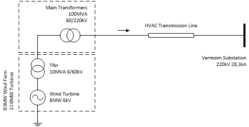Figure 1. Layout of the Wind Farm

As shown on the figure above, the authors chose to use a 220kV link to the shore, given the rated power of the wind farm and the existing transmission infrastructure on that region. REN’ Vermoim Substation located approximately 40km from the district capital Oporto was the onshore Point of Connection (PoC). The tables 1 and 2 present, respectively, the characteristics of the wind farm and the ratings at the given substation (at the 220kV busbar).

Table 1. Characteristics of the Wind Farm

Nr. Units	SN-Turb [MW]	SN-Farm [MW]	LLink [km]
10	8	80	200

Table 2. Short-circuit ratings at Vermoim 220kV Busbar

SCC MAX [MW]	SCC MIN [MW]	ICC MAX      [kA]	ICC MIN   [kA]
10.7	8.3	28.3	21.7

2.2.  Characteristics of the HVAC Link

The usage of insulated cables as the means to transmit power in HVAC is understandingly common. Nonetheless, offshore (submarine) applications have a different behavior that ultimately and most importantly, significantly reduce the acceptable distance of application. Limitations, such as high charging current and higher Ferranti effect [8], are widely known, the model must allow for the analysis of several scenarios, with real-time adjustment and performance assessment, still ensuring a less time-consuming computation of each one.

There are two main cable-sizing criteria, which are the rated voltage and admissible temperature [8] and the model is based on this simplification.

The nominal current is given directly by the rating of the wind farm whereas the fault current value is given at the HV OHL-bay at the onshore substation as it is the most significant contributor in case of short-circuit at the PoC. Both allow for an estimation of the minimum cable cross-section [7]:

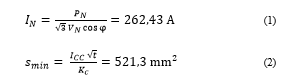Where t represents the fault-clearance time.

Having this as a reference, and given the cable standardization, a core section of 630mm² shall be selected. The OHL and cable will be selected having such as a reference. The upstream grid is not taken into consideration on the analysis (meaning the onshore PoC is assumed a PV-type node).

3. Software Implementation

3.1.  Electrical Line-equivalent Model

When in comparison between lumped-sum or parabolic line-equivalent models, the differences are significant. In the case of OHL, the parabolic components of the equivalent are almost unitary, which allows for simplification and a lump-sum provides acceptable results [8].

In cable applications in general, the wave impedance is higher and as so the propagation constant decreases, resulting in non-unitary trigonometric components. These models compute the opposite-end results based on a linear and concentrated impedance section, the propagation speed is not taken into account (which drives from the simplification itself).

In order to proper translate the effects of submarine cable applications, the model has to take into account the influence of the propagation speed and the geometrical distance. An accurate model has to take effectively into account the distribution and variation of the parameters along the line, being therefore distance and transmission velocity- dependent (which lastly decreases for a higher cable length).

This knowledge is widely applied in very-fast transient analysis for atmospheric discharges or other high-velocity voltage and/or current variations on transmission lines. An x section of the line is presented in Figure 2.

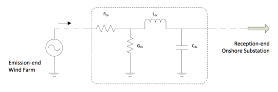Figure 2. Infinitesimal section of the cable ( [9], adapted)

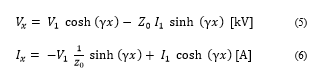
As the results of that equivalent scheme are much more accurate, the respective equations (3) to (6) are used on the MATLAB model. These, on the first approach, provide a distance-based analysis of a given transmission link in regards to estimated voltage and current:

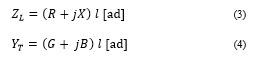The voltage and current for x distance are given by:

All data shown on the GUI (hence plot options) are also based on a set of calculations detailed on the script. The calculations are performed for any given initial conditions, non-related to any previous tests – although a multi-set analysis can be provided, as shown on sections 4 and 5.

3.2.  Model Design

The necessity to address a multitude of scenarios to draft earlier conclusions has led itself to the conclusion that a software, rather than casual calculation, had to be taken into practice. The development of a fast and custom-made tool to the analysis the design of HV transmission lines led the authors almost directly to the implementation of a GUI-based MATLAB model.

That allowed for the creation of a versatile and digital tool, which allows for a fast and straightforward verification, given a set of any initial conditions, if power transmission via a selected line (or power cable) is acceptable in technical terms. And, the model spans virtually to any range of, not only cables, but voltage, current, power factor or distance.

The possibility of checking a certain scenario in real-time and in on-hand is another plus, possible via the multitude of adjustments possible on the model itself, with instantaneous calculation and results. As the GUIDE is, basically, the user-friendly window of MATLAB C-based programming, also quite an user-friendly design was achieved.

In practical terms, the model operates by taking into account a set of transmission line conditions – stored on pre-loaded, yet adjustable .XLS sheet, of OHL and cables, then applies the equivalent model earlier addressed (section 3), and computes all the results that illustrate the steady-state operation of a given transmission “line”. That includes voltage, current, no-load voltage & current, voltage drop, efficiency (losses evaluation), power factor, stability, surge impedance level (SIL) and model parameters (Z_L & Y_T).

3.3.  Model Key Advantages

The segmentation and expandability of the model can be defined as two of the most important characteristics. All the information used and key features, aside from cables, are actually .XLS-based. The model starts and loads-up the majority of its functionalities with reference to the options and fields set on the configuration Excel sheets.

Features such as the stress parameters used for the calculation – further on shown – or the actual regulations, such as voltage or reactive power boundaries, can be adjusted with ease. The model also loads using acceptable and recommended voltage, current, power factor and distance values, further facilitating the usage. The plot section, on the other hand, allows for the simultaneous visualization of three different calculation windows, thus allowing the user do address a scenario in a much more complete manner.

Finally, the information provided has a key focus. As said, the ability to implement the line-equivalent is wide-spread in literature. The difference is to provide such information and the data outcomes in simpler yet much more complete manner. That information is provided to the user using overlay layers on the results plotted, and may include operational boundaries, compensation expectations, stress-range distance pin-pointing, or even, simultaneous calculation results – for example, for difference one-end power factors. The summary of the available results is shown on Table 3.

Table 3. Available Results of the Model

Ref	Description
1	Powerline Voltage
2	Powerline Current
3	No-load Current
4	No-load Voltage
5	Voltage Angle
6	Current Angle
7	Voltage Phase Displacement
8	Current Phase Displacement
9	Active Power
10	Reactive Power
11	Apparent Power
12	Transmission Losses
13	Transmission Efficiency
14	Voltage Drop
15	Power Factor
16	Tan-Phi
17	Stability Limits (Pe-Phi)
18	Voltage Drop (DV-PF)
19	SIL (impedance)
20	SIL (apparent power)
21	Longitudional Impedance
22	Transverse Admittance

The critical factors that guide the operational ranges are shown in Table 5. Generically (and, in fact changeable), the critical factors are presented based on two conditions: “C” (meaning Critical, for 80% of target) and “F” (for Failure, or 100% of target value). Other conditions may apply as mention on Table 5. The numbers refer to the references and 80/100 thresholds can be adjusted as the intention of the user with minor core programming adaptation.

Once again, model design is as simple yet flexible and expandable as possible. The majority of the reference and configuration-data is XLS-based and new features are easy to implement. The same can be done for the (line) data, as the routine reads any given organized sheet and performs the calculation. After the automated analysis is complete, the user can make a search, distance or variable-dependent, for a value-at-point or given location of the “line”.

Figure 3. General overview of the settings window of the model

As observed in Figure 3, the real-time interface is possible via the adjustable sliders – which adapt the basic parameters. Re-calculation is done fast and automatically after any change on those. The advantages of a tailor-made GUI model span for other areas. The plotting windows included have been adapted to allow for the online setting of the units to be used: International system (SI) units, per-unit (P.U.) or %-based results.

The adjustment of the ranges and precision of the axis is adjusted directly on each respective axis line. Exporting is also made directly from the working plotting window, allowing for quick integration on written reports. This is, once more, allowed by a strong background interface with .XLS files, and further on, with facilities such as additional interfaces, adaptation, parameter-variation mode and export facilities, are all intricate on the model.

Table 4. Critical Factor References for Model

Ref	Variable Checked	Slope	Critical Value	Failure Value
1-4	Line Voltage	>=	REN regulations
5-8	Line Voltage	<=	REN regulations
9	Line Current	>=	Thermal limit of cable
10-13	No-load Voltage	>=	REN regulations
14-17	No-load Voltage	<=	REN regulations
18	No-load Current	>=	50%	100%
19	Reactive Power	>=	40%	50%
20	Losses	>=	40%	50%
21-22	Voltage Angle	>=	±30º	±40º
1-4	Line Voltage	>=	REN regulations
5-8	Line Voltage	<=	REN regulations
9	Line Current	>=	Thermal limit of cable
10-13	No-load Voltage	>=	REN regulations
14-17	No-load Voltage	<=	REN regulations

What is also worth mentioning is the ability to automatically see the stress ranges on a color-coded plot-overlay for any given calculation. These ranges are recognized and the maximum operating distances are identified. Ranges are loaded based on the Portuguese regulations (e.g. REN) and those can also be adjusted.

For a comparison to be made on different transmission solutions a simulation is made on a 220kV air-insulated single-circuit single-pole transmission line. The rated voltage is selected taking once again into account the grid topology at the PoC.

4. Evaluation of Air-Insulated Connection

4.1.  Parameter Calculation

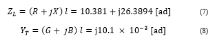
The overall manufacturer-issued characteristics of such cable, later on introduced on the MATLAB model, are shown on Table 5. The maximum active power output is stationed at 80MW (having a cos j of 0,85 lag). The matrix therefore can be calculated as presented in equations (7) and (8).

Table 5. Characteristics of the simulated Overhead Line

UN [MW]	r [mΩ/km]	L [mH/km]	C [nF/km]
220.0	77.3	1.362	8.553

These values are automatically calculated on the model.

4.2.  Experimental Results

Computation is done assuming the reference data at the reception-end (onshore PoC). The simulation of the voltage and current at the emission-end of the line are shown on Figures 4 and 5. Ultimately, the results confirm the reliability of the model with existing accurate OHL-analysis data [9]. The calculation method is than transposed to an offshore (submarine) framework, as presented on section 5.

Figure 4. Powerline voltage simulation (220kV OHL)

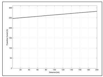Figure 5. Powerline current simulation (220kV OHL)

The analysis of the submarine cable, being the focus, shall include much more significant data, however all being supported on the positive result of the voltage & current simulation shown on these two test plots.

5. Evaluation of Submarine Cable Connection

5.1.  Parameter Calculation

The analysis of the submarine cable, hence parameter calculation, is done on the same basis as before. The cable data obtained from the manufacturer (ABB) is presented in Table 6. Cables are laid in a single pole linear and evenly distributed along the seabed.

Table 6. Characteristics of the simulated Submarine Cable

VN        [kV]	IN       [A]	Size [mm2]	R     [Ω/km]	L       [mH/km]	C          [μF/km]
220	600	630	0.04935	1.4000	0.1600

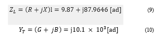Once again, these are automatically calculated on the model. Equations (5) and (6) apply for the calculation of all data plotted, including the calculation of the ABCD equivalent model parameters.

5.2.  Voltage & Current Results

The operation, critical failure ranges can be seen on the figures shown. The reference for criticality/failure leads back to the REN regulations on the voltage boundaries. The same is shown on the current plot. A distance shorter than 100km is also sufficient to show the relevant information yet that range facilitates the condensation of data on the plot snapshot.

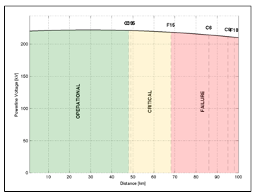Figure 6. Powerline voltage simulation (220kV Submarine Cable)

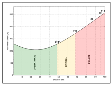Figure 7. Powerline current simulation (220kV Submarine Cable)

The emission-end (WF) values are 210kV (Fig. 6) and 513A (Fig. 7). As it can be verified, the voltage drop reaches close to 5%. As for the current, it’s final value is around two times the initial current value at the reception. This allows for an insight of one of the most important downsides of cables – the charging effect.

As far as the current values are concerned, the high capacitive characteristics of the submarine cable, lead to a significant increase of the line’ current and emphasize the reactive power flow. This not only increases the power losses along the line but also confirms that cable solutions are not feasible after 30-50km [10] alongside theoretical information available.

5.3.  Voltage Drop on Underground & Submarine Cables

As a basis of comparison, Figures 8 and 9 include the voltage drop along transmission cables using underground (8) and submarine (9) solutions. Evidently, as expected, the reduction of the voltage is much more significant on the second option.

The authors emphasize that, on both land and sea cables, the voltage drop encountered is actually a voltage rise along the line, due to the capacitive characteristics of the cables themselves. This has to be later on compensated on the WF-side, forcing the generators to operate under very low voltages.

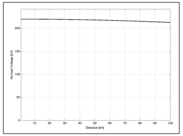Figure 8. No-load voltage simulation (220kV Underground Cable)

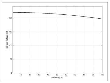Figure 9. No-load voltage simulation (220kV Submarine Cable)

The inductance value has a tremendous influence on the voltage and current behaviour of the transmission line, but with more focus on the first one mentioned. Aside from the voltage decline – and as addressed earlier – with a higher impact, the charging and Ferranti effects are evaluated for this particular cable.

5.4.  Charging Current & Ferranti Effect

The charging and Ferranti effects are the two most distinguishable plots which can be made from the behavior of insulated cables (both underground and submarine. The high capacitance of these cables leeds to a early increase on the current flow and therefore the transmittable power is severely restricted. No-load current, based on the F18 marker on the plot, is actually the failure cause of the cable under investigation.

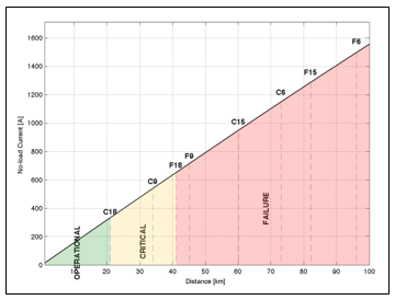Figure 10. No-load current simulation (220kV Submarine Cable)

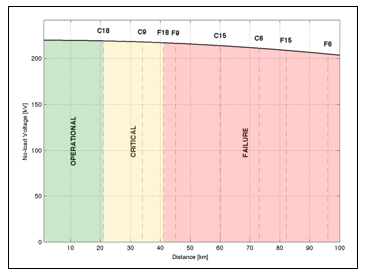Figure 11. No-load voltage simulation (220kV Submarine Cable)

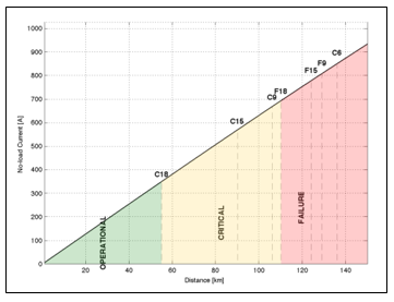Figure 12. No-load voltage simulation (220kV Submarine Cable)

When compared to the equivalent underground cable included on the examples of the model, the differences are tremendous. The effect on the submarine option is almost 100% more. The operation of such “large capacitor” under no-load conditions also translates onto a voltage increase along the same cable – as shown previously on Figure 9.

5.5.  Power Factor & Reactive Power Results

The behaviour of the power factor for a given section of the transmission cable is highly dependent on the initial conditions, especially the reception-end (PoC) power factor. For that reason, this section also includes a multi-scenario analysis, thus allowing for a better understanding of such impact.

A very high drop on the power factor is observed (close to 50% of the initial value), to a minimum of 0,44. Due to the increasing current, the active power still increases. However, it is the reactive power which increases the most, leading again to the failure of this setup for more than 70 kilometres (F15).

What is also verified is that, up to a certain distance, the capacitive characteristics of the line help to compensate for the inductive grade of the load (0,8 lag). Once the characteristics of the transmission line match the PoC, there is an inversion on the slope.

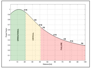Figure 13. Power factor simulation (220kV Submarine Cable)

What is also verified is that, up to a certain distance, the capacitive characteristics of the line help to compensate for the inductive grade of the load (0,8 lag). Once the characteristics of the transmission line match the PoC, there is an inversion on the slope. After a certain distance (around 25km), the cable is actually acting as a reactive power provider. This fault is not triggered because, in percentage, it is still below the 50% threshold shown on Table 4.

What can also be understood from Fig. 8 is that the unitary power factor is obtained for a distance just under 15km. Despite failure only occurs after 40km (once more confirmed by literature), because the line has a significantly higher capacitance than the OHL, it acts much like a very large capacitor, consuming a highly capacitive current during operation. After 100km, the current required is about the same as the rating of the load (Figure. 7).

These results are quite conclusive on the balance that must be met. They also provide a further understanding on how much the compensation solutions must be tailor-made and real-time adjustible to proper ensure the safety of the link.

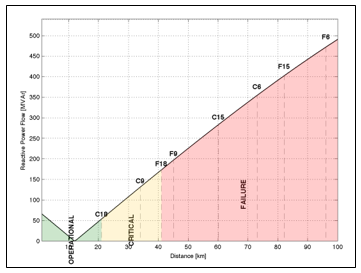Figure 14. Reactive Power simulation (220kV Submarine Cable)

5.6.  Losses & Efficiency

Losses are a significant part of the link evaluation. The model includes several paths to illustrate the losses. Two of the options are provided here: transmission efficiency and transmission (Joule) losses, plotted in Figures 15 and 16.

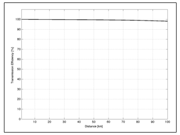Figure 15. Transmission efficiency simulation (220kV Submarine Cable)

The efficiency remains under an acceptable range (above 90%). This easily confirms that the insulated cables have equivalent losses to the OHL, whereas the capacitive restrictions are the actual restrictions to the operation of these AC offshore links.

In a way, due to the higher inductance value, the capacitive current is not so high and Joule losses are slightly reduced. Nevertheless, the values commented are still very high and above acceptable boundaries. Losses are also similar to the equivalent land cable.

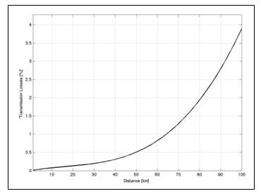Figure 16. Transmission losses simulation (220kV Submarine Cable)

5.7.  Voltage, Current & Displacement Angles

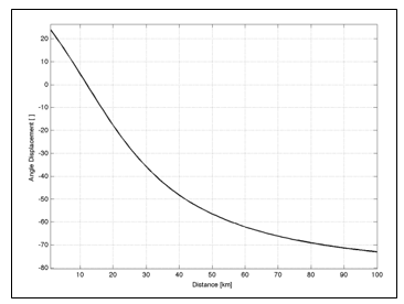Figure 17. Angle displacement simulation (220kV Submarine Cable)

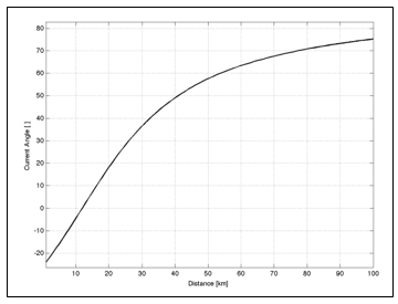Figure 18. Current angle displacement simulation (220kV Submarine Cable)

The plot of the voltage and current angle displacements between the two ends of the cable is also a clear sign that, above the mentioned 40km, the cable is working under unacceptable operational conditions. The voltage is assuming a strongly capacitive characteristic. A comparison on the voltage angle variation for equivalent land and submarine cables is on Fig. 19.

Figure 19. Angle displacement simulation (220kV Submarine Cable)

The angle and power factor values provide once more a good understanding path of the range of operation of the submarine link. The tendency of both curves is much alike the equivalent land cable. The power factor, here stated at 0,33 continues to be very low, inducing that the cable still behaves like a large capacitor. The analysis performed for the land cable, in order to assess the natural load and connectable distance is now demonstrated.

5.8.  Variation of Cable Loading

With an inherit highlight of one of the additional major features of the model, this part presents the effects on the variation of the cable loading – current at the reception-end, once more, in regards to power factor and line current. The results are shown next. Hatches were disable to facilitate the visualization.

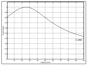Figure 20. Power factor (load variation) simulation (220kV Submarine Cable)

If the impedance of the load is below the line’s impedance, it means that the active power delivered is higher than the natural power for such voltage / cable. Land cables, which have a lower inductance and higher capacitance, are usually operated below their natural power [9], which is calculated, for this particular case, as follows:

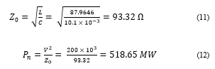However, subsea cables are characterized to a much higher inductance value, thus changing that approach. With a higher rating yet under the thermal capabilities of the cable, such cable can operate and obtain better operational values.

Addressing the effect on the cable loading, both in terms of rated power, but also, in terms of power factor is crucial. The higher the current provided by the wind farm, a negative shift of the peak power factor occurs, thus leading to conclude that the cable has a wider operation range if the loading (current) is close to its rated value.

On the other hand, for an equivalent unitary capacitance, the sea cables have a much higher inductance, which for certain ranges and loads, it can help to compensate the power factor variation on the line.

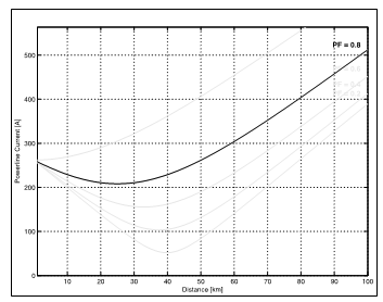Figure 21. Current (load variation) simulation (220kV Submarine Cable)

          As shown on Fig. 14, the lower the power factor of at the WF-side, the lower the current fed from the WF itself. On the other hand, the impact on the reference voltage is important. The voltage and current angles are also exposed to significant changes due to the variation of the initial power factor. The results are included on Figures 16 and 17.

This means that the lower the power factor (lag) is assumed, the voltage and current angles have smother slopes. This translates the mutual “compensation” between the power factor and the PoC and the capacitive characteristics of the long submarine cable.

For the current angle, the values at the end of scale (full distance) do not pose significant differences. But, if the center range of the angle curve is observed, it is clear that the acceptable operational boundary is improved with such power factor decrease.

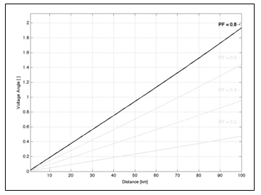Figure 22. Voltage angle (load variation) simulation (220kV Submarine Cable)

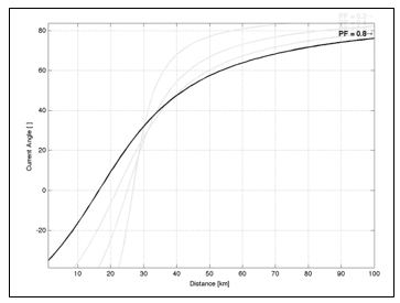Figure 23. Current angle (load variation) simulation (220kV Submarine Cable)

Bearing in mind the purely academic approach for this – as cables used differ for distinct nominal voltages, what the model quickly provides is a framework on how an higher voltage can facilitate higher power flow. This is addressed via the SIL plot shown in Fig. 18.

The results on Fig. 16. further prove that model designed, as the conclusion, voltage increase allows for a higher SIL rating of the cable, which is aligned with the bibliography. The main result however is the easiness how this is selected on the GUI, by using the “Label” and “Freeze” capabilities. This allows the user to shown several identified scenarios {voltage, current, power factor, distance and compensation}.

Regardless, the what the authors conclude is that is now much easier, both in an academic or (risks measured) practical manner, to quickly assess the best conditions for which an AC offshore link should be designed. One route for the improvement of these results (links) is compensation.

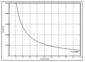Figure 24. Current (load variation) simulation (220kV Submarine Cable)

6. MATLAB Compensated Results

The analysis of the compensated transmission cables is done still using the multi-scenario approach. As provided earlier, as the parameter changed in each scenario is automacally overlayd on the plot itself, concludes are easily drafted.

6.1.  Estimation of Compensation

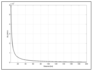Figure 25. SIL simulation (220kV Submarine Cable)

Based on the results of the reactive power and considering a unitary power factor load, it is possible to estimate the rating of a shunt reactive compensation system – previously decided by the authors after execution a several scenario investigations using the same model. The reactive power is included in Figure 14 whereas the SIL (loading) evaluation is provided in Figure 25.

Given such and based on the experimental values shown on Fig. 16, 265MVAr was put into experiment. The effects on the voltage and power factor, two of the main images of the cable, are shown on the next section.

6.2.  Voltage after Compensation

What is immediately observed is a shift of the stress (failure) point earlier identified, thus a clear improvement on the operational range. The reactive power at the emission, for nod distance, represents the full rating of the compensation.

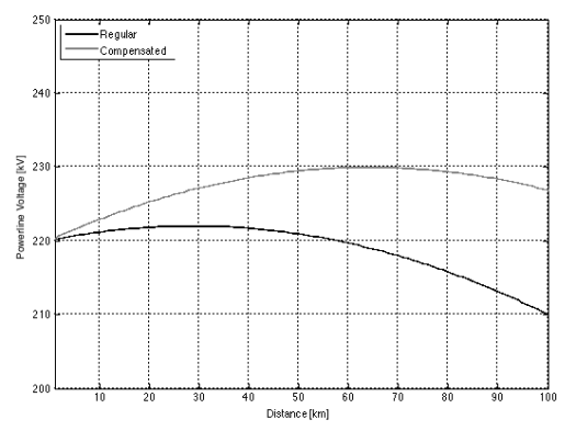Figure 26. Voltage (after compensation) simulation (220kV Submarine Cable)

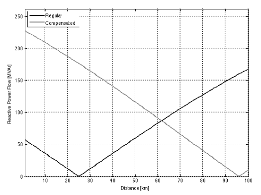Figure 27. Current (after compensation) simulation (220kV Submarine Cable)

The GUI interface easily presents several scenarios, without going through a labour-intensive calculation routine. Taking once more the approach of adapting the cable loading (current at the reception-end), additional conclusions can be gathered (as provided on Figures 27 and 28).

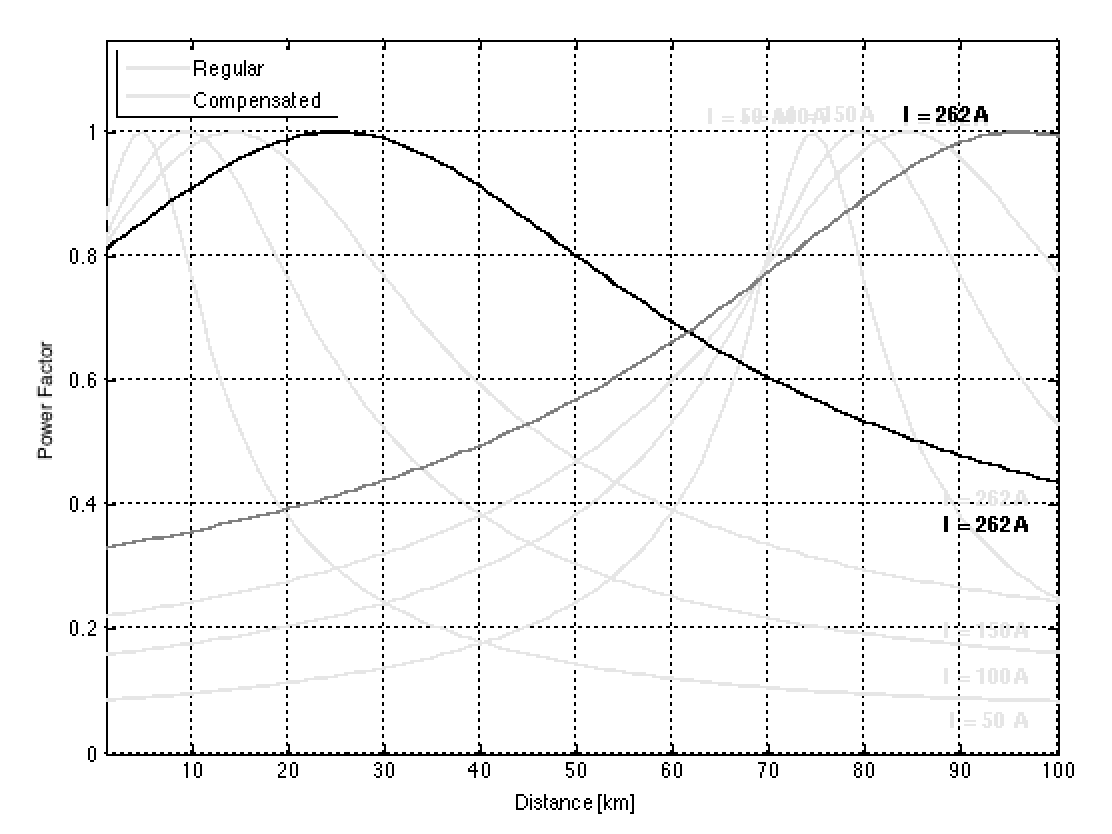Figure 28. Power factor (load variation after compensation) (220kV Cable)

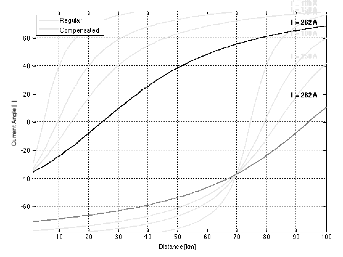Figure 29. Current (load variation after compensation) (220kV Submarine Cable)

Voltage, reactive power and the power factor are now within perfectly acceptable boundaries, for the full 100km length.  The power factor must be analysed depending on the point of connection of the compensation system, eventually using a split-off between the two ends.

Especially after the introduction of compensation, several loading scenarios have to be taken into account, once more, taking advantage of the GUI-model. For lower loading scenarios, the compensation system output has to be reduced or, eventually, taken out of service. Otherwise, what is identified in Figs. 19 and 20 is a clear overcompensation for a load drop (current). Nowadays, online FACTS systems effectively support the reactive power flow demanded by large-scale offshore wind farms. Although not addressed on this paper, once again, the model points to a quick rough estimation of a possible compensation solution.

7. Final Remarks & Conclusion

The authors firmly believe that this computational simulation tool is an important guide on the assessment of HVAC transmission links, especially for offshore applications such as wind farms.

As expected, the submarine cables presented the authors with the worst operational conditions from all the three options addressed on this document. The high inductance of such cables, mostly due to their type of insulation, introduces serious limitations, which translate in very short feasible distances. If this was the baseline for the investigation, the model as shown that the conclusions are obtained experimentally with ease.

The authors believe that the results shown before allow for a sufficient and accurate perception of the problematic associated with large HVAC transmission lines. The results were conclusive, with minor errors taking into consideration the objective proposed. So much more can be done in a further stage.

There is however still room for further improvement on the existing model, addressing topics such as different types of compensation of lines or introducing further characteristics of the line, of course, that can affect the line’s behavior in some way.

The compensation system here studied also has some limitations, namely in terms of type (only fixed-step compensation is addressed) and in terms of distribution, eventually on several stages of the cable or transmission line. Future developments of the model should address this topic and allow for a more broad study of compensation effects.

The work can also extended and applied across other industries, such as Oil&Gas – for offshore energy supply to platforms and interplatform energy safety-grids. The goal of providing a safe and reliable tool, able to provide link estimations in a window of seconds to minutes was achieved.

Conflict of Interest

The authors declare no conflict of interest.

Acknowledgment

The authors thank EDP Distribution (the Distribution System Operator in Portugal). This work also has been once more partially supported by the Portuguese Foundation for Science and Technology under projects grants PEst-OE/ EEI/UI308/2014 and UID/EEA/00066/2013.

1. T. A. Antunes, P. J. Santos and A. J. Pires, “HVAC transmission restrictions in large scale offshore wind farm applications,” in 2017 11th IEEE International Conference on Compatibility, Power Electronics and Power Engineering (CPE-POWERENG), Cadiz, Spain, 2017.
2. H. Holttinen, J. Kiviluoma, J. McCann, M. Clancy, M. Millgan, I. Pineda, P. B. Eriksen, A. Orths and O. Wolfgang, “Reduction of CO2 emissions due to wind energy – methods and issues in estimating operational emission reductions,” in Power & Energy Society General Meeting, 2015 IEEE, Denver, USA, 2015.
3. International Renewagle Energy Association, “The Power to Change: Solar and Wind Cost Reduction Potential to 2025,” IRENA, 2016.
4. B. Gustavsen and O. Mo, “Variable Transmission Voltage for Loss Minimization in Long Offshore Wind Farm AC Export Cables,” in IEEE Transactions on Power Delivery , 2016.
5. Siemens AG, Wind Turbine SWT-8.0-154: Technical Specifications, Hamburg: Wind Power and Renewables Division, 2016.
6. Siemens AG, “Powered by partnership: Sustainable solutions for your offshore wind power project,” 2016.
7. ABB, “XLPE Cables up to 420kV,” 2013.
8. D. Moura, Técnicas de Alta Tensão – Curso Introdutório, Lisboa: Técnica – Revista de Engenharia, Lda., 1980.
9. J. P. Sucena Paiva, Redes de Energia Eléctrica, Uma Análise Sistémica, 2nd Edition ed., vol. 1, I. Press, Ed., Lisbon: IST Press, 2007.
10. Siemens, “High Voltage Direct Current Transmission: Proven Technology for Power Exchange,” Siemens AG, Alemanha, 2011.

(Click Here)

(Click Here)