1. Introduction

Atmospheric conditions such as windshear continue to be considered as a source of potentially severe consequences. They are dangerous for aircraft during landing or take-off, because the wind gusts can occur at relatively low altitudes. Nevertheless, windshear is also dangerous during the cruise flight phase because it can lead to violation of the prescribed flight level.

In view of threats related to wind disturbances, there is permanent interest in designing robust aircraft guidance and control schemes (possibly for use with autopilots). The related question consists in finding safety domains, i.e. sets of initial states from which the control problem can be solved in the case of worst wind disturbance whose components lie in a known range.

There exist a large number of works devoted to the problem of aircraft control in the presence of severe windshears. In particular, papers [1–6] address the problem of aircraft control during take-off in windshear conditions. In works [1] and [2], the wind velocity field is assumed to be known. It is shown that open loop controls obtained as solutions of appropriate optimization problems provide satisfactory results for rather severe wind disturbances. Nevertheless, it is clear that the spatial distribution of wind velocity cannot be measured with appropriate accuracy, and therefore feedback principles of control design are more realistic. Different types of feedback controls are proposed in papers [3–6]. In [3], the design of a feedback robust control is based on the construction of an appropriate Lyapunov function. Robust control theory is used in [4] to develop feedback controls stabilizing the relative path inclination and (in [5] and [6]) for the design of feedback controls stabilizing the climb rate.

An approach based on differential game theory (see e.g. [7]) is presented in paper [8] in connection with the problem of landing. A high dimensional nonlinear system of dynamic equations is linearized and reduced to a two-dimensional differential game using a transformation of variables. The resulting differential game is numerically solved, and optimal feedback controls are constructed and tested in the nonlinear model against a downburst.

Another method, also based on differential game theory, is used in papers [9] and [10] to find feedback controls that are effective against downbursts. This approach assumes the computation of the value function, which is a viscosity solution (see. e.g. [11] and [12]) of an appropriate Hamilton-Jacobi equation. The numerical implementation utilizes dynamic programming techniques described in [13] and [14]. The case of known wind velocity field as well as the case of unknown wind disturbances are considered.

Recent investigations [15] and [16] utilize a method (see [17]) for the fast computation of rough approximations of solvability sets in linear conflict control problems. Using techniques of sequential linearization, this method is applied to nonlinear aircraft dynamics to design an appropriate control for take-off in the presence of downbursts.

The current paper addresses the problem of retaining trajectories in an appropriate flight domain (AFD) corresponding to the cruise flight phase (cf. [18] and [19]). Viability theory (see e.g. [20]) provides numerical methods (see e.g. [21], [22], and the Appendix) for finding the viability kernel, i.e. the largest set of initial states lying in the AFD from which viable trajectories emanate. More precisely, it includes all initial states for which there exists a feedback control that generates trajectories remaining in the viability kernel for all possible admissible wind gusts. In the case where the initial state does not belong to the viability kernel, there exists a method of designing a wind disturbance such that all trajectories violate the AFD for all possible controls.

As for wind conditions, it is assumed that only bounds on the wind velocity components are imposed. The dynamics of the aircraft will be considered as a differential game (cf. [9] and [10]) where the first player chooses control inputs, whereas the second player forms the worst wind disturbance. It is assumed that the first player is able to measure the current state vector, whereas the second player can measure both the current state vector and the current control (“future” values are not available) of the first player. Therefore, the second player may use the so-called feedback counter strategies (see [7]).

The current paper has common features with the open-access publication [23] concerning the model description and solution method. It should be noted that the publication [23] is mainly focused on theoretical fundamentals of the differential game approach. Regarding computational results, paper [23] formulates a problem of constructing the viability kernel in seven dimensions and performs several steps of the algorithm to show its feasibility. In contrast, the current paper addresses aspects of implementation on large scale grid computers and completely solves the above mentioned seven-dimensional problem including simulation of optimal trajectories.

The paper is structured as follows:

Section 2 outlines a point-mass aircraft model describing the vertical motion of a generic modern regional jet transport aircraft. The model is closely related to the one described in paper [23]. The difference consists in a more clear method of deriving the dynamics equations.

In Section 3, state constraints related to the cruise flight phase are formulated, and the corresponding computed viability kernels are demonstrated through their three-dimensional sections. Additionally, trajectories yielded by an optimal feedback strategy, working against an optimal control of the disturbance, are shown. It should be noted that an optimal control of the disturbance can be constructed either as counter or pure feedback strategy because the so called saddle point condition holds for the differential game under consideration.

Section 4 outlines some aspects of parallel implementation of the computational method on a supercomputer system. The parallelization principles and data flow inside and between compute nodes are sketched. The novelty of our approach and comparison with existing software tools are discussed.

Section 6 (Appendix) briefly outlines the concept of differential games and viability kernels. Grid schemes for the computation of them are sketched. The details can be found in [23].

2. Model equations

In this section, a point-mass model representing the vertical motion of a generic modern regional jet transport aircraft is considered. Table 1 introduces euclidean coordinate systems (COS) that are necessary to compute the forces exerted on the aircraft. The origins of COSs are located either at the aircraft gravity center (CG) or at a fixed reference point (O) on the earth surface.

Table 1: Aircraft coordinate systems

COS	Index	x-axis	Origin
Local Kinematic Aerodynam.	N K A	Parallel to the Earth’s surface (xN ) and upwards (zN ) −−→ In direction of VK −−→ In direction of VA	O CG CG
Thrust	P	In positive direction of the symmetry axis of the turbine (aft looking forward)	CG
Body Fixed	B	In direction of the nose and in the symmetry plane of the aircraft	CG

Here, V~_K and V~_A are kinematic and aerodynamic aircraft velocities, respectively. The angles defining the relationship between the coordinate systems are the following (see also Figure 1):

αK	the kinematic angle of attack,
αA	the aerodynamic angle of attack,
γK	the kinematic path inclination angle,
σ	the thrust inclination angle.

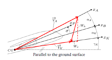Figure 1: Aircraft coordinate systems and angles

Matrices for the transformations K → N (Kinematic to Local ), A → B (Aerodynamic to Body), B → K (Body to Kinematic), and P → B (Thrust to Body) are

defined as follows:
“ MNK = sin(γKK)) cos(γ	−sin(γK)#, cos(γK)
“ MBA = sin(αAA)) cos(α	−sin(αA)#, cos(αA)
“ MKB = sin(αKK)) cos(α	−sin(αK)#, cos(αK)
“cos(σ) MBP = sin(σ)	−sin(σ)# . cos(σ)

The position propagation is given in the local coordinate system (N), whereas the translation dynamics

are derived in the kinematic coordinate system (K).

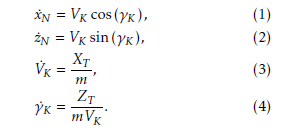Here, X_T and Z_T denote the components of the total force F~_T represented in the kinematic coordinate system (K), and the notation m stands for the aircraft mass. As usually, F~_T comprises aerodynamic, propulsion, and gravitation forces:

F~_T = F~_A +F~_P +F~_G.

Aerodynamic forces. They are defined as follows:

F~A = MKBMBA“CCDL # 21ρVA2S,

where C_D and C_L are the drag and lift coefficients, respectively, ρ = ρ(h) is the air density (depends on the altitude), V_A the aerodynamic velocity, and S the wing reference area.

The lift and drag coefficients C_D(α_A,M) and C_L(α_A,M) are taken in the form:

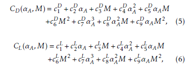
where the coefficients c_i^D and c_i^L, i = 1,…9 are determined from least square fitting to experimental data.

The absolute value, V_A, of the aerodynamic velocity can be derived using its relation to the kinematic velocity V~_K in the Local frame (N) and the wind velocities W_x and W_z in the x_N and z_N directions, respectively. Therefore,

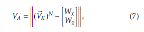 and finally, using the matrix M_NK, this implies the formula

V_A² = (V_K cosγ_K − W_x)² +(V_K sinγ_K − W_z)².

The aerodynamic angle of attack α_A is computed as follows:

where u_A and w_A are x_B and z_B-components of the aerodynamic velocity, respectively.

The Mach number M is defined as follows:

where c is the speed of sound, κ the adiabatic index for air, R the gas constant for ideal gases, and T (h) the temperature of air at the altitude h. See [23] for more details.

Propulsion Forces. Thrust forces are modeled considering a two-engine setup. Thus,

where δ_T ∈ [0,1] is the thrust setting, and the functions f_V and f_γ are approximated similar to formulas (5) and (6), with δ_T instead of α_A. See [23] for more details.

Gravitation Force. For a simple gravitational model with constant acceleration g, the corresponding force is computed as:

where M_KN is the inverse (transpose) of M_NK.

The following two equations are added to the dynamics (1)-(4) to exclude jumps in the controls:

Furthermore, the following equations produce smoothing of wind disturbances:

 where the time constant, k_w, is chosen as k_w = 1s⁻¹.

3. Problem setting and simulation results

Problem. The model consists of equations (2), (3), (4), (8), and (9). Thus, the state vector has seven variables: z_N , V_K, γ_K, α_K, δ_T , W_x, and W_z. The controls are associated with the rate of the angle of attack, α_eK, and the rate of the thrust setting, δ_eT . Their instantaneous changes are permitted. The disturbances are now associated with the artificial variables W_fx and W_fz that are inputs of the filters (9). Thus, the physical wind components W_x and W_z do not exhibit instantaneous jumps.

The following constraints on the controls and disturbances are prescribed:

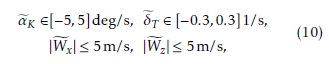|Wfx| ≤ 5m/s, |Wfz| ≤ 5m/s, and the following state constraints are imposed: h_N := z_N − h₀ ∈ [−90,90]m, V_K ∈ [100,200]m/s, |γ_K| ≤ 10deg, (11) α_K ∈ [0,16]deg, δ_T ∈ [0.3,1],

where h₀ = 10000m being the cruise flight altitude.

Additionally, the state constraints |W_x| ≤ 5m/s and

|W_z| ≤ 5m/s hold automatically because of equations (9) and the constraints (10).

In the numerical construction, the box [−100,100]× [90,210]×[−15,15]×[−4,20]×[0.2,1.2]×[−6,6]×[−6,6] of the space (h_N ,V_K,γ_K,α_K,δ_T ,W_x,W_z) was divided in 200×120×30×24×14×12×12 grid cells. The sequence of time steps, {δ_{`</sub>}, was chosen as δ<sub>`} ≡ 0.01, and the computations were performed until V_{`</sub><sup>h</sup><sub>+1</sub> − V<sub>`}^h ≤ 10⁻⁵ for all grid nodes. Totally, 4471 steps of the algorithm (19) were done. The computation has been done on the SuperMUC system at the Leibniz Supercomputing Centre of the Bavarian Academy of Sciences and Humanities. The computation was distributed over 100 compute nodes with 16 cores per node, which is regarded as “middle task” on the SuperMUC system. The runtime was about 40 h.

Figures 2-4 show different three-dimensional sections of the seven-dimensional viability kernel. Figures 5-7 respectively demonstrate the same threedimensional sections and the corresponding projections of two optimal trajectories emanating from points lying in the viability kernel. The start point of trajectory 0 lies near to the boundary of the viability kernel, whereas trajectory 1 starts from a point lying deep inside of the viability kernel. The trajectories are computed when the control uses its optimal feedback strategy, and the disturbance utilizes its optimal counter feedback strategy (see the Appendix). The time step size used in the simulation of the trajectories was equal to 0.01. It is seen that the trajectories go to their attraction cycles and remain there. The simulation time interval is [0,15min]. Figure 8 shows a three-dimensional section of a smaller viability kernel corresponding to the shrinkage of the state constraints (11) by the factor 0.7. The corresponding three-dimensional projection of two optimal trajectories are shown. It is seen that the disturbance can keep trajectory 0 outside the reduced viability kernel because the start point lies outside of it.

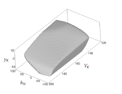Figure 2: A three-dimensional section of the viability kernel: α_K = 8, δ_T = 0.65, W_x = 0, and W_z = 0. αK

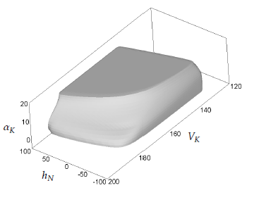Figure 3: Another three-dimensional section of the viability kernel: γ_K = 0, δ_T = 0.65, W_x = 0, and W_z = 0. δ_T

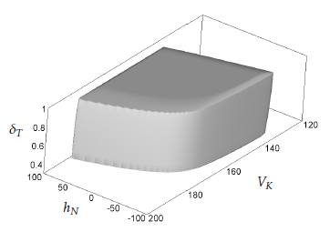Figure 4: One more three-dimensional section of the viability kernel: γ_K = 0, α_K = 8, W_x = 0, and W_z = 0. γK

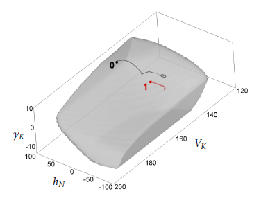Figure 5: The section from Figure 2 and projections of two trajectories generated by an optimal feedback strategy of the control and an optimal counter feedback strategy of the disturbance. The start points are marked with bullets.

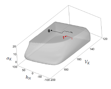Figure 6: The same section as in Figure 3 and projections of the same two trajectories as in Figure 5.

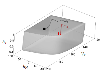Figure 7: The same section as in Figure 4 and projections of the same two trajectories as in Figure 5.

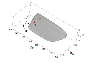Figure 8: The section (α_K = 8, δ_T = 0.65, W_x = 0, and W_z = 0) of a smaller viability set corresponding to the shrinkage of the state constraints by the factor of 0.7. Projections of the same trajectories as in in Figure 5 are shown. Since the start point 0 does not belong to this viability set, the disturbance can keep the trajectory outside of it.

4. Implementation Aspects

4.1.  Grid Computing, Parallelization and Scaling

We use a self developed software code to implement the algorithms of the grid scheme outlined in Appendix 6.3. The code is parallelized using a mixed MPI/OpenMP technique. The first two dimensions of the grid are decomposed, whereas the other dimensions remain unmodified. A compute node cartesian topology (see Figure 9) is then created such that each compute node corresponds to a grid cylinder. Additionally, each grid cylinder is supplied with ghost nodes that allow us to compute divided differences

(18) used e.g. in the algorithm (19). In Figure 9, the lines connecting the compute nodes show the data flow supported by MPI. The parallelization inside of each compute node (i.e. inside a grid cylinder) is supported by OpenMP.

The problem considered in this paper deals with a seven-dimensional grid of 200×120×30×24×14×12×12 cells. Each of the first two dimensions was divided into 10 parts. Thus, there were 100 grid cylinders, each of size 20 × 12 × 30 × 24 × 14 × 12 × 12, plus the necessary ghost grid nodes. Therefore, the required memory per compute node was equal to about 8GB.

Our observations show a good scaling behavior (see

Table 2). The results were obtained for the problem of computing the viability kernel in five dimensions on a 200 × 120 × 30 × 24 × 14 grid. The relative speedup normalized to 32 cores and absolute timing of 30000 steps are shown.

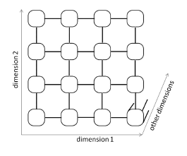Figure 9: Compute node cartesian topology used in our applications.

Table 2: Scaling behavior of the code

# of	Linear	Observed	Wall	Perfor-
cores	predic-	scaling	time	mance/core
	tion of scaling		[h]	[GFlop/s]
32	1	1	9.7	20
128	4	3.5	2.8	17.5
1600	50	38	0.25	15.2

4.2. Novelty of the method used

This paper utilizes a new method for computing viability kernels, which is based on the results of paper [21]. It is proven in [21] that the viability kernel is the Hausdorff limit of the sets {x : V (x,t) ≤ 0} as t → −∞, where V (x,t) is the value function (see [7]) of a state constrained differential game .

The numerical implementation of this method requires a theoretical basis and a stable numerical procedure for the treatment of transient Hamilton-Jacobi equations related to differential games with state constraints. Such a theoretical basis is given in paper [13] where the conventional conditions for viscosity solutions are modified to account for state constraints. This theoretical background is numerically implemented in [13] and [14], which results in monotone stable grid scheme (17) and (19). This enables us to perform a large number of time steps, usually several thousands.

Another new feature is that the corresponding software code is deeply parallelized using hybrid MPI/OpenMP techniques and adapted to run on a supercomputer system. Moreover, diverse modified variants of the code, based on sparse representations of grid functions, are tested.

4.3. Comparison with existing software

The well known software for solving Hamilton-Jacobi equations is the Level Set Method Toolbox (LSMT) described in [24]. This tool is really appropriate for solving rather general problems. However, it is not indicated in the manual whether the LSMT can compute viability kernels for differential games with state constraints. Moreover, according to the manual, the LSMT is not parallelized, whereas our software runs on a multi-node system.

5. Conclusion

This investigation shows that methods of differential games theory and viability theory can by applied to nonlinear aircraft models to investigate potential control abilities in the presence of wind disturbances. The new feature of our approach is the consideration of viability kernels for differential games. Feedback strategies of the players can be found from limiting grid “value functions” defining viability kernels (cf. Appendix). It is important that the amount of stored data is relatively small, which permits to implement the computed feedback strategies on a flight simulator. Further research will be focused on the treatment of models with more state variables, which will allow us to consider more realistic problems. Moreover, accounting for additional sources of uncertainty such as sensor errors or modeling uncertainties is planned.

Acknowledgment

This work was supported by the DFG grants TU427/2-1 and HO4190/8-1. Computer resources for this project have been provided by the Gauss Centre for Supercomputing/Leibniz Supercomputing Centre under grant: pr74lu.

6. Appendix

This section briefly summarizes a method presented in [23] for computing viability kernels. Such a summary should help to provide a self-contained presentation.

6.1. Differential game

Consider a conflict control system with the autonomous dynamics Here; x stands for the state vector; u and v denote control inputs of the first and second players, respectively; and the compact sets P and Q describe constraints imposed on the control and disturbance variables, respectively. Further, it is assumed that all functions of x have global properties. For example, the right-hand side f is supposed to be bounded, continuous, and Lipschitzian in x on Rⁿ × P × Q.

In the following, it is assumed that the Isaacs saddle point condition minmaxhs

is true for all s ∈ Rⁿ and x ∈ Rⁿ. Note that this condition holds for the problem under consideration because controls and disturbances are additively separated in the model equations.

6.2. Viability kernel

For any v ∈ Q, consider the differential inclusion

Let G ⊂ Rⁿ be a compact set such that G = intG, this set will play the role of the state constraint. Let T be an arbitrary fixed time instant, and N = (−∞,T ] × G. For any subset W ⊂ N and any time instant t ≤ T , define the time section of W through the relation W(t) := {x ∈ Rⁿ : (t,x) ∈ W }.

Definition 1 (u-stability property [7]) A set W ⊂ N is called u−stable on (−∞,T ] if for any position (t_∗,x_∗) ∈ W, for any time instant t^∗ ∈ [t_∗,T ], for any fixed v ∈ Q, there exists a solution x(·) of the differential inclusion (14) with the initial condition x(t_∗) = x_∗ such that (t^∗,x(t^∗)) ∈

The next proposition is taken as a basis of the definition of viability kernels.

Proposition 1 [see [21] for the proof] Let W be a maximal u-stable subset of N = (−∞,T ] × G. If W(t) ,∅ for any t ≤ T , then the set is nonempty, and W(t) → K in the Hausdorff metric as t → −∞. The set K is called the viability kernel of G and denoted by V iab(G).

Proposition 2 Let t >¯ 0 be an arbitrary time instant, and x_∗ ∈ V iab(G). Then there exists a feedback strategy A(x) of the first player such that all trajectories yielded by A and started at t = 0 from x_∗ remain in the set V iab(G) for all t ∈ [0,t¯] and any actions of the second player. If x^∗ < V iab(G), then there exists a feedback strategy B(x) and a time instant t_f such that all trajectories yielded by B and started at t = 0 from x^∗ violate the state constraint G for t > t_f and any actions of the first player.

6.3. Grid method for computing viability kernels

For the implementation of numerical method, it is convenient to represent viability kernels as level sets of an appropriate function. Let G_λ be a family of state constraint sets defined by the relation

where a continuous function g is chosen in such a way that, e.g., G₀ being the desired state constraint. It is necessary to construct a function V representing the viability kernels as follows:

Such a function can be computed as a limiting solution, as t → −∞, of an appropriate Hamilton-Jacobi equation arising from conflict control problems with state constraints (see [13]). A grid approximation of V is computed as described below (cf. [21], [22], and [23]).

Let δ > 0 be a time step length, and the tuple

h := (h₁,…,h_n) defines space step sizes. Set |h| := max{h₁,…,h_n} and introduce the following upwind operator defined on grid functions related to the discretization h:

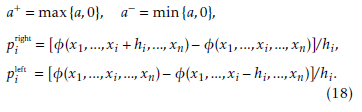
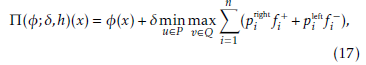with f_i being the components of f (x,u,v), and a⁺ = max{a,0}, a⁻ = min{a,0},

Let {δ_{`</sub>} be a sequence of positive reals such that δ<sub>`} → 0 and ^P. Consider the following grid scheme: `+1   h;δ`,h,gh, V0h = gh, ` = 0,1,…,

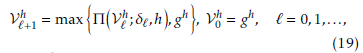where g^h is the restriction of g to the grid defined by h.

It can be proven that V_`^h monotonically converges point-wise to a grid function V^h, and this function define approximations of the viability kernels according to formula (16), see [23] for more details.

Remark 1 In (17), the operation min_u∈_P max_v∈_Q can be changed for max_v∈_Q min_u∈_P to obtain almost the same result. The difference tends to zero with |h|. The proof follows from the fact that the original operator (17) and the modified one satisfy the same consistency condition (see [13]) involving the following Hamiltonian H:

H(x,p) := maxminhp,f (x,u,v)i = minmaxhp,f (x,u,v)i. v∈Q u^∈P             u^∈P v∈Q

Numerical computations confirm this observation.

6.4. Control design

This section outlines one of possible methods of control design. Consider the grid scheme (19) assuming that ` is large enough so that the required approximation is

The optimal control u and the worst disturbance v(u) at the current state x of the game can be found as solutions of the following program: u,v → minu max^LhhV_`^hix +τf (x,u,v). (20)

Here, L^h is an interpolation operator (see e.g. [14]) defined on the corresponding grid functions, and τ being a parameter which should be several times larger than the time step size of the simulation procedure to provide some stabilization. Note that the function V_`^h can be transferred to a sparse grid (see e.g. [25] and [26]), which may essentially reduce the storage space. The disadvantage of such a technique is a certain loss of accuracy and a slower performance.

Remark 2 As it is described above, the second player uses the so-called feedback counter strategies, i.e. functions of x and u, where u being the current control action of the first player. Since the saddle point condition (13) holds, the theory of differential games says that the second player can achieve the same result using pure feedback strategies, i.e. functions of x. For example, a near optimal strategy of the second player can be obtained as a solution of the problem

u,v ^→ maxv∈Q minu^∈P ^LhhV_`^hix +δf (x,u,v),

see also Remark 1. Thus, the both players achieve optimal results using pure feedback strategies.

Remark 3 If u and v appear linearly in the right-hand side of (12), then min and max operations in (17) and (20) can be computed only over extreme points of the sets P and Q respectively. This can be proven using the same arguments as in Remark 1.

Remark 4 If x₀ being a start point of the game, then x₀ lies in the approximate viability kernel defined as:

and all trajectories approximately remain in this set. However, if the second player works non-optimally for a while, then, most likely, V_{`</sub><sup>h</sup>(x(t¯)) < V<sub>`}^h(x₀) for some t >¯ 0, and therefore, the state vector x(t¯) lies now in the smaller viability kernel

{x ∈ Rn : V`h(x) ≤ V`h(x(t¯))}.

Thus, faults of the second player improve the result of the first one.

Conflict of Interest

The authors declare no conflict of interest.

1. Miele, T. Wang, W.W. Melvin, “Optimal take-off trajectories in the presence of windshear” J. Optimiz. Theory App., 49(1), 1–45, 1986. https://doi.org/10.1007/BF00939246
2. Miele, T. Wang, W. W. Melvin, “Guidance strategies for near-optimum take-off performance in windshear” J. Optimiz. Theory App., 50(1), 1–47, 1986. https://doi.org/10.1007/BF00938475
3. H. Chen, S. Pandey, “Robust control strategy for take-off performance in a windshear” Optim. Contr. Appl. Met., 10(1), 65–79, 1989. doi:10.1002/oca.4660100106
4. Leitmann, S. Pandey, “Aircraft Control under Conditions of Windshear” in C. T. Leondes (ed.) Control and Dynamic Systems, vol. 34, part 1, 1–79, 1990. Academic Press, New York.
5. Leitmann, S. Pandey, “Aircraft control for flight in an uncertain environment: takeoff in windshear” J. Optimiz. Theory App., 70(1), 25–55, 1991. https://doi.org/10.1007/BF00940503
6. Leitmann, S. Pandey, E. Ryan, “Adaptive control of aircraft in windshear” Int. J. Robust Nonlin., 3(2), 133–153, 1993. doi:10.1002/rnc.4590030206
7. N. Krasovskii, A. I. Subbotin, Game-Theoretical Control Problems, Springer, 1988.
8. S. Patsko, N. D. Botkin, V. M. Kein, V. L. Turova, M. A. Zarkh, “Control of an aircraft landing in windshear” J. Optimiz. Theory App., 83(2), 237–267, 1994. https://doi.org/10.1007/BF02190056
9. D. Botkin, V. L. Turova, “Application of dynamic programming approach to aircraft take-off in a windshear” AIP Conference Proceedings, 1479, 1226–1229, 2012. https://doi.org/10.1063/1.4756373
10. D. Botkin, V. L. Turova, “Dynamic programming approach to aircraft control in a windshear” in V. Krivan, G. Zaccour(eds.) Advances in Dynamic Games. Annals of the International Society of Dynamic Games, vol. 13, 53–69, 2013. Birkh¨auser, Cham. https://doi.org/10.1007/ 978-3-319-02690-9_3
11. G. Crandall, P. L. Lions, “Viscosity solutions of Hamilton- Jacobi equations” T. Am. Math. Soc., 277(1), 1–47, 1983. https://doi.org/10.1090/S0002-9947-1983-0690039-8
12. I. Subbotin, Generalized Solutions of First Order PDEs: The Dynamical Optimization Perspective, Birkh¨auser, 1995.
13. D. Botkin, K.-H. Hoffmann, N. Mayer, V. L. Turova, “Approximation schemes for solving disturbed control problems with non-terminal time and state constraints” Analysis, 31(4), 355–379, 2011. https://doi.org/10.1524/anly.2011.1122
14. D. Botkin, K.-H. Hoffmann, V. L. Turova, “Stable numerical schemes for solving Hamilton–Jacobi–Bellman–Isaacs equations” SIAM J. Sci. Comput., 33(2), 992–1007, 2011. https://doi.org/10.1137/100801068
15. Martynov, N. Botkin, V. Turova, J. Diepolder, “Real-Time Control of Aircraft Take-Off in Windshear. Part I: Aircraft Model and Control Schemes” in 25th Mediterranean Conference on Control and Automation (MED), Valletta Malta, 277–284, 2017. IEEE. doi:10.1109/MED.2017.7984131
16. Martynov, N. Botkin, V. Turova, J. Diepolder, “Real-Time Control of Aircraft Take-Off inWindshear. Part II: Simulations and Model Enhancement” in 25th Mediterranean Conference on Control and Automation (MED), Valletta Malta, 285–290, 2017. IEEE. doi:10.1109/MED.2017.7984132
17. K. Kostousova, “On target control synthesis under setmembership uncertainties using polyhedral techniques” in C. P¨otzsche, C. Heuberger, B. Kaltenbacher, F. Rendl (eds.) System Modeling and Optimization, vol. 443, 170–180, 2014. Springer-Verlag, Berlin-Heidelberg. https://doi.org/ 10.1007/978-3-662-45504-3_16
18. Seube, R. Moitie, G. Leitmann, “Aircraft take-off in windshear: a viability approach”. Set-Valued Anal., 8(1-2), 163–180, 2000. https://doi.org/10.1023/A:1008786811464
19. M. Bayen, I. M. Mitchell, M. K. Osihi, C. J. Tomlin, “Aircraft autolander safety analysis through optimal control-based reach set computation” J. Guid. Control Dynam., 30(1), 68–77, 2007. https://doi.org/10.2514/1.21562
20. P. Aubin, “A survey of viability theory” SIAM J. Control Optim., 28(4), 749–788, 1990. https://doi.org/10.1137/0328044
21. D. Botkin, V. L. Turova, “Numerical construction of viable sets for autonomous conflict control systems” Mathematics, 2(2), 68–82, 2014. doi:10.3390/math2020068
22. D. Botkin, V. L. Turova, “Examples of computed viability kernels” Trudy Inst. Mat. i Mekh. UrO RAN, 21(1), 306–319, 2015. http://mi.mathnet.ru/eng/timm1190
23. Botkin, V. Turova, J. Diepolder, M. Bittner, F. Holzapfel, “Aircraft control during cruise flight in windshear conditions: viability approach” Dyn. Games Appl., 7(4), 1–15, 2017. https://doi.org/10.1007/s13235-017-0215-9
24. Mitchell, A Toolbox of Level Set Methods, UBC Department of Computer Science Technical Report TR-2007- 11, 2007. https://www.cs.ubc.ca/˜mitchell/ToolboxLS/ toolboxLS-1.1.pdf
25. Zenger, “Sparse grids” in Hackbusch, W. (ed.) Parallel Algorithms for Partial Differential Equations. Notes on Numerical Fluid Mechanics, vol. 31, 241–251, 1991. Vieweg, Braunschweig/ Wiesbaden. doi: 10.1002/zamm.19920721115
26. Pfl¨uger, “Spatially Adaptive Sparse Grids for Higher- Dimensional Problems”, Dissertation, Verlag Dr. Hut, M¨unchen, 2010.

(Click to view)

(Click to view)