1. Introduction

We live in the era of ‘Big Data’, where a vast amount of structured, semi-structured and unstructured data are being generated at an ever-accelerating pace and can be mined to obtain valuable information. The most commonly used approach to process this kind of data is to aggregate raw data into large datasets, probably extend them with metadata, and then apply machine learning and/or artificial intelligence algorithms in order to identify repeatable patterns [1]. Artificial neural networks are a rapidly developing category of machine learning structures that give computers the capability to learn without being explicitly programmed to perform specific tasks. They consist of different layers for analyzing and learning data. Each layer consists of a large number of highly interconnected processing elements (neurons), working together to learn from previous data in order to solve specific problems by making proper decisions.

Boltzmann Machine (BM) is a typical example of a neural network structure. BMs are probabilistic Markov Random Field models that use a layer of hidden variables to model a distribution over input variables, called visible variables. In general, learning a Boltzmann machine is a computationally demanding process. However, the learning problem can be simplified by imposing restrictions on the network topology, which leads to Restricted Boltzmann Machines (RBMs)[2]. RBMs are structured as bipartite undirected graphs, which results to efficient inference implementation, and are particularly capable of learning complex features. The last few years, many applications based on RBMs have been developed to cover a large variety of learning problems, such as image classification, speech recognition, collaborative filtering and so on. One such example application is the recognition of handwritten digits. Learning an RBM corresponds to fitting its parameters, so that the distribution represented by the RBM models the distribution underlying the training data, handwritten digits in this case [3]. The storage resources and the time required not only to train an RBM but also to make real-time predictions on new coming data increases exponentially with the number of parameters. Thus the development of a handwritten digit recognition application on a single user machine is a non-trivial task.

Nowadays, cloud computing solutions provide new capabilities to users and enterprises for processing their data remotely in high performance servers. Users do not have to invest in information technology infrastructure, reducing the need for advanced hardware at the user side. In addition, cloud providers specialized in a particular area, such as image processing, can bring advanced services to a single user, complex services that are not easily afforded by individual users. Another important benefit is the high processing rate that can be achieved when a high performance server is used for processing requests from multiple independent users.

In this work, which is an extension of the work originally presented in [4] and [5], we exploit the vast amount of resources provided by cloud computing along with the high computation capabilities offered by hardware accelerators in order to build a complete cloud-based engine that can be used in real-time handwritten digits recognition (HDR). The engine collects images from multiple sources over the cloud and processes them as fast as possible resulting in high processing rate. The high processing rate is achieved by using a powerful hardware accelerator that implements a number of neural networks operating in parallel. A major advantage of the proposed engine is that the training of the neural networks is not only performed once during initialization of the system, but it is also fed with new images periodically, thus improving the accuracy of the prediction results. The engine is presented in detail in the sections that follow.

Section 2 gives an overview of existing implementations, especially on handwritten digits recognition. Section 3 analyzes Restricted Boltzmann Machines and how they can be modified in order to be used to solve classification problems, such as image recognition. Section 4 presents the architecture and the functionality of the proposed cloud-based computing server. Section 5 highlights the communication interface between the server and the hardware accelerator. Section 6 describes in detail the implementation of the neural networks, with emphasis on the architecture of the dedicated hardware accelerator. A complete system prototype was developed, which is presented in Section 7. Experimental results that demonstrate the system performance in terms of processing rate for both implementations are also presented.

2. State of The Art

The scientific area of automatic handwriting recognition is of great interest for both academia and industry. Existing algorithms are so efficient in learning to recognize handwritten digits that they are used, for example, by post offices to sort letters and banks to read personal checks. MNIST is the most widely used dataset for studying handwritten digit recognition [6]. State-of-the-art models that present accuracy results in the range of 0.35% down to 0.23% error rates are based on large Convolutional Neural Networks (CNNs), either in the form of a deep single network optimized with various training techniques or as a committee of many smaller networks [7], [8], [9]. The best results so far, 0.21% error rate, have been claimed by an approach based on regularization of neural networks using DropConnect [10].There is a listing of the state-of-the-art results and links to the relevant papers on the MNIST and other datasets collected by Rodrigo Benenson [11].

The disadvantage of CNNs is that they are very resource-demanding and their training and inference procedures are extremely time-consuming. As the amount of data increases, machine learning moves to the cloud and big clusters of high-performance servers are used for providing real-time results. Most works mainly deal with implementing the training procedure by using distributed servers over the cloud ([12], [13]) or by using higly scalable FPGA implementations ([14], [15]). In this work, a high performance computing engine that accepts images from multiple clients over the cloud and classifies them with high accuracy is presented.

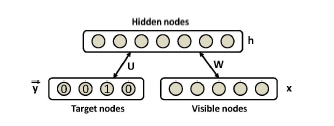Figure 1: Discriminative RBM modeling the joint distribution of inputs and target classes.

3. Classification Restricted Boltzmann Machines

Restricted Boltzmann Machines are usually used as feature extractors for other learning algorithms or as initializers for deep feedforward neural network classifiers, not as standalone classifiers. However, authors in [16] have proposed a discriminative variant of RBMs that can be used autonomously in classification tasks offering good performance results. The bipartite undirected graph of such an RBM is illustrated in Figure 1. Given a training set D_train = {(x₁,y₁),…,(x_i,y_i),…,(x_D,y_D)}, where i denotes the i-th example of the set consisting of an input vector x_i and the corresponding target class y_i ∈ {1,…,C}, we use the specific RBM to model the joint distribution between a layer of N hidden variables h = (h₁,…,h_N ), usually referred as features, and the observed variables (x,y). It is a parametric model where the parameters Θ = (W,b,c,d,U) represent the following:

• W: Weights matrix between x and h
• U: Weights matrix between e_y and h
• b,c,d: Respective biases of x, h and e_y and e_y = (1_i=y) for i ∈ {1,…,C} the ‘one out of C’ vector representation of y.

We consider the binary version of the model where each node, hidden or visible, may be in one state, ON or OFF. A node adopts a new state as a probabilistic function of the states of its neighboring nodes and the weights on its links to them. It stands:

X

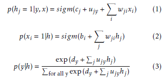where sigm(x) = 1/(1 + e^−x) is the logistic sigmoid function.

After the model has been trained, the conditional probability p(y|x) is used for classification. The conditional probability p(y|x), can be computed using p(y|x) = argmin(F(y,x)):

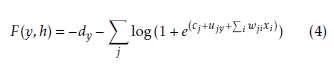where F(y,h) is called free energy.

In order to train an RBM to solve a particular classification problem, an objective has to be defined that the learning procedure will try to minimize for all examples in the dataset D_train. It is possible to choose among various different objective functions, but generally the following three are used [17]:

• Generative Training Objective
• Discriminative Training Objective
• Hybrid Training Objective

3.1. Generative Training Objective

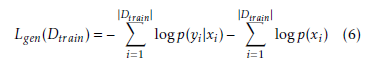
Given that the model defines a value for the joint probability p(x,y), a natural choice for a training objective is the generative objective:

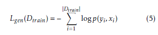Computing logp(y_i,x_i) and its gradient with respect to any RBM parameter Θ is intractable. Fortunately it has been shown that the gradient can be well approximated using the Contrastive Divergence estimator. The analytical computation is replaced by an estimate at a sample generated after a limited number of Gibbs sampling steps, with the sampler’s initial state for the visible variables set at the training example (x_i,y_i). A single Gibbs sampling iteration is usually sufficient to learn a meaningful representation of the data [18]. Then, this gradient estimate can be used in a stochastic gradient descent procedure for training. A pseudocode of the procedure is given in Algorithm 1, where γ is the learning rate. Usually, the weights (W,U) are initialized using small random values, while the biases (b,c,d) are initially zero. Ideally, RBMs require parameter updating after each single example, but mini-batch updating can be also used. However, in order to ensure fast model convergence, the batch size should remain relatively small.

Algorithm 1 RBM Training over (x,y) using 1-step

Contrastive Divergence

Input: w_ij for all training samples (x,y) do

1. Calculate p(h = 1|x,y) for all hidden nodes Sample the hidden distribution < h₀ >
2. Perform Gibbs sampling for k steps (k=1):

Calculate p(x|h₀) for all visible nodes and p(y|h₀) for all target nodes

Sample the visible distribution < x_k > and the target distribution < y_k >

Calculate p(h = 1|x_k,y_k) for all hidden nodes

Sample the hidden distribution < h_k >

3. Calculate gradients:

gW =< h_k > ∗ < x_k > − < h₀ > ∗x gU =< h_k > ∗ < y_k > − < h₀ > ∗y gb =< x_k > −x gc =< y_k > −y gd =< h_k > − < h₀ >

4. Update weights and biases:

W ⁰ = W − γ ∗ gW U⁰ = U ⁻ γ ^∗ gU b⁰ = b ⁻ γ ^∗ gb c⁰ = c ⁻ γ ^∗ gc d⁰ = d ⁻ γ ^∗ gd

end for

3.2. Discriminative Training Objective

The generative training objective can be decomposed as follows:

This means that the RBM classifier will dedicate some of its capacity at modeling the marginal distribution of the input only. Since classification is a supervised learning task and we are only interested in obtaining a good prediction of the target given the input, we can ignore the unsupervised part of the generative objective and focus on the supervised part. So, the discriminative training objective is defined as:

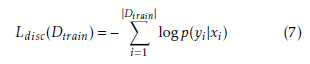The most important advantage using this training objective is that it is possible to compute exactly its gradient with respect to the RBMs parameters for each example (x_i,y_i). For the various model parameters it stands:

• For Θ = (b) the gradient is zero, since the input biases are not involved in the computation of p(y|x).

3.3. Hybrid Training Objective

The effectiveness of both generative and discriminative approaches on various problems has been studied and it has been shown that they have quite different properties. For classification tasks, adding the generative training objective to the discriminative training objective is a way to regularize the second one. To adapt the amount of regularization, the Hybrid Training Objective can be used:

where the weight α of the generative part can be adjusted based on the performance of the model on a validation set.

3.4. Training using MNIST

In this work, RBMs were applied on a classic classification problem, handwritten digit recognition using the MNIST dataset [6]. MNIST is a large database of handwritten digits, commonly used for training various image processing systems. The database is also widely used for machine learning and pattern recognition methods. The original MNIST dataset is used here, which contains 60,000 training and 10,000 test examples with 28×28 grey-scale images corresponding to all 0-9 digits. This is a multiclass classification problem, where the number of target classes is 10. Before final integration, the best parameters for the RBM model should be selected. These parameters include the number of hidden nodes N, the learning rate γ, which training objective is minimized, the generative weight α, as well as the batch size bs. For that reason, a complete Matlab simulation model was developed and the effect of the different parameters was studied using a validation set. It should be noted that for the specific problem, Hybrid Training led to faster convergence.

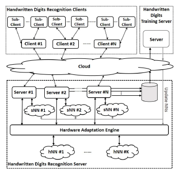Figure 2: The HDR Computing Engine Architecture

4. HDR computing engine architecture

Based on Classification RBMs, a high performance computing engine able to serve a large amount of real-time requests for detecting the correct values of handwritten digits was implemented. This is a complete infrastructure with multiple entities specially designed either for training of already accumulated data or for real-time classification of multiple new images. Concerning the neural networks implementation, both software modules and dedicated hardware accelerators were developed.

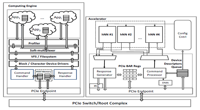Figure 3: Hardware Adaption Engine – Interfacing with the HDR hardware accelerator

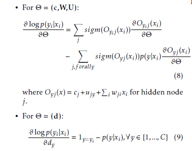
The architecture of the proposed HDR computing engine is shown in Figure 2. This engine accepts requests from various clients from the cloud and processes them in real-time. The system is composed of three basic entities, which are a) Handwritten Digits Recognition clients, b) Handwritten Digits Recognition servers and c) Handwritten Digits (HD) training server. The HDR clients can either be individual clients or sets of sub-clients that are serviced by an HDR client that combines their requests in a single data stream. Each HDR client is associated with a dedicated HDR server. The number of HDR servers that are executed at any given time is variable and is determined by the number of HDR clients that are supported. The main advantage of the proposed architecture is that it does not use a set of predefined parameters but it uses the information of a large number of clients for continuously updating the weights and biases of the HDR algorithm, achieving high accuracy for a given complexity. The HD training server is responsible for updating these parameters. More specifically:

HDR Clients: A two-way TCP/IP connection [19] between every HDR client and a dedicated HDR server is established. They exchange variable size data blocks, serviced either partially for better latency or as a whole block for better processing rate.

HDR Servers: When a request for a new connection arrives, a new HDR server thread is activated. Each thread receives bunches of images by its client and stores them temporarily to its local memory. Each HDR server may accept different types of requests from its client. The requests may differ at the number of images per block, the image size, i.e. 16×16 or 28×28 pixels, and pixel information coding (1 bit per pixel, 8 bits per pixel etc.). The server uses either its built-in processing capability to serve the requests, which means that the neural network is implemented in high-performance software, or forwards them to a dedicated hardware accelerator.

HD Training Server: The HD training server receives data and performs the training of the RBM neural networks. The data are forwarded to the HD training server either during initialization of the system or periodically during normal operation. In the latter case, the HDR servers send a random subset of images along with the information regarding the digit recognition. After training, the HD training server is responsible for sending the updated parameters, weights and offsets, back to all neural networks.

Concerning the neural network implementation there are three possible configurations.

• Software-only Configuration: a software NN (sNN) is initialized per HDR thread. Each

NN accepts images by its corresponding thread, classifies them and returns the predicted digits.

• Hardware-only Configuration: a small number of NNs implemented in hardware (hNN) is available to all server threads and is shared among them. The execution time is much smaller compared to the software implementation and that results to much higher processing rate. The hardware accelerator is based on a powerful FPGA board attached to the computing engine’s CPU using a high-speed interface, either native PCIe Gen 3.0 with more than 1 GBps useful transfer rate [20] or the Coherent Accelerator Processor Interface (CAPI)

[21]. An entity called Hardware Adaptation Engine (HAE) provides a seamless interface between the server threads and the accelerator. This entity is described analytically in the next section. Each HDR server does not use a specific hNN but whichever is available. The hardware accelerator may consist of multiple FPGA boards and/or GPUs. Although this architecture is significantly more efficient, in the case of a heavy workload, each hNN may have to process a huge bunch of images. In this case, a hybrid configuration is most preferable.

• Hybrid Configuration:      the          images    are          still processed by the hardware accelerator (hNNs) but when the processing delay exceeds the software execution time, then the sNNs start receiving some of the images for classification.

5. Hardware Adaptation Engine

The HDR servers receive bunches of images from their clients and store them in a FIFO at the input of HAE. Each HDR server has its own dedicated FIFO. HAE is responsible for forwarding these images for recognition to the hardware accelerator. HAE consists of multiple functional units that are shown in Figure 3. Initially, the Profiler decides the next block of images that has to be forwarded to the Soft-multiplexer. The number of images per block is selected so that the total system performance is maximized. The Soft-multiplexer interfaces with the hardware accelerator through Block/Character device drivers. The drivers and the accelerator communicate through shared host memory areas. When the images have been processed by the accelerator, a response with the digits values is fed back to the proper HDR server. A more detailed description of the HAE functional units follows.

5.1. Profiler

It is responsible for selecting the next block of images that has to be handled by the Soft-multiplexer. The Profiler decisions depend on the number of pending commands and the total response statistics (execution time etc.). The HDR servers inform the Profiler about their pending commands, while the Soft-multiplexer provides timing information regarding command execution. Initially, the Profiler selects the commands of the next block using either a round-robin or a static algorithm with fixed priorities. When enough statistics have been collected, dynamic allocation that takes into consideration the current load is feasible.

5.2. Soft-multiplexer

It makes the basic calls for interfacing with the Character/Block device drivers (e.g. open, close, pwrite, pread, ioctl etc). The Soft-multiplexer processes the selected block, extracts the commands and forwards them to the drivers. After receiving a notification for the completion of a command, the Soft-multiplexer forwards a response to the corresponding server thread. The soft-multiplexer also informs the Profiler about the execution time of each bunch of images.

5.3. Character/Block Device Driver

It is responsible for transferring the data from user space to kernel space and vice versa, for address translation and interrupt handling. The commands are associated with a data structure, in the form of a descriptor, which is the basic information provided to the hardware accelerator. The Device Driver activates the Command and Response Handler for forwarding commands and receiving the respective responses from the accelerator. The Command Handler accepts commands, creates the descriptors and stores them in a shared host memory area (Host Descriptors Queue). Each descriptor may contain one or more commands, associated with data from the same or different HDR servers. When a block of descriptors has been processed and their responses are ready, the accelerator sends an MSI-X Interrupt to notify the Response Handler that responses are stored in another shared host memory area (Responses Queue). The Response Handler decodes each response and forwards the corresponding results to the Soft-multiplexer.

At the accelerator’s side, the Command Processor is responsible for accessing the descriptors at the host’s main memory and transferring them into accelerator’s local memory (Device Descriptors Queue). It decodes the descriptors, transfers the requested images using a DMA engine and feeds any available hNN. When the image processing has been completed the Response Generator prepares the responses that contain the classified digits, stores them in the Responses Queue and sends an interrupt to the Device Driver.

6. Neural Network Implementation

For better exploitation of the hardware resources, images of 16×16 pixels, with 1 bit/pixel, are used. This can be achieved by proper prefiltering and scaling, without affecting significantly the total system’s accuracy. For this image size each hNN uses less hardware resources, thus enabling more hNNs to be integrated in the given accelerator resources, while the accuracy is only slightly reduced. These images are generated by the original ones after proper filtering and optimum threshold application. The pre-processing takes places at the client side before transmission. Before moving to the actual neural network implementation, a theoretical analysis of certain parameters regarding the prediction procedure is necessary.

6.1. Theoretical Analysis

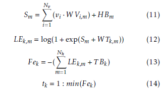
As aforementioned, classification is based on the calculation of free energy [22], given by (4). For implementation purposes this equation is rearranged as follows:

where N_h is the number of hidden nodes, N_t the

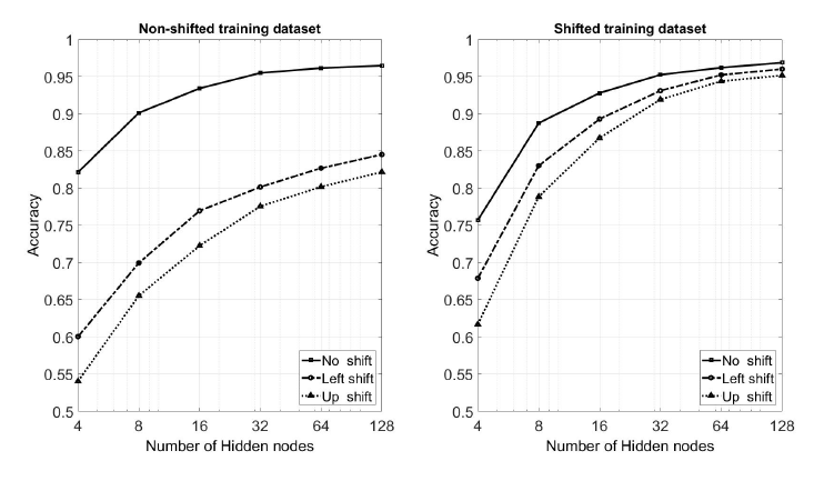Figure 4: The influence of different training datasets on classification’ s accuracy.

number of target nodes, m ∈ [1,N_h], k ∈ [1,N_t], v_i is visible node i, h_m is hidden node m and t_k is target node k. Fe_k is the free energy of target node k. Regarding the weights and biases, V B_i are the biases of visible nodes, T B_k are the biases of target nodes, HB_m are the biases of hidden nodes, WV are the weights between visible and hidden nodes and WT are the weights between target and hidden nodes.

In order to study more thoroughly the accuracy of the proposed implementation and validate its effectiveness under a broader set of images, the initial dataset was extended with shifted versions of the original images. More specifically, four additional datasets were created, each one being a shifted copy of the initial one. The images were shifted to the left, right, up or down by a single pixel. In this way, the final dataset is a superset of the original one. Training was performed using both datasets, the original non-shifted one and, to keep the dimensions the same, a randomly selected collection of 60,000 images from the shifted dataset.

Figure 4 shows the effect of the training dataset on the classification accuracy of the model, when it is applied on three individual datasets, the original test dataset with the non-shifted images, the test dataset with the images that have been shifted left by one pixel and the test dataset with the images that have been shifted up by one pixel. As expected, the use of the shifted version for training leads to better overall accuracy, except in the case of the original dataset and for a small number of hidden nodes. This is explained by the fact that an RBM can model fewer dependencies when it includes a small number of hidden nodes, thus being subject to overfitting on the training dataset. Similar results can be taken for the datasets with the one-pixel right and down shifting.

Figure 4 also helps to specify the number of hidden nodes that will be used in both the software and hardware implementations of the neural network. It is obvious that the choice of 32 hidden nodes is a satisfactory trade-off between accuracy and complexity. By choosing 64 hidden nodes the accuracy improves only 2.2%, while the hardware complexity increases almost 8 times.

6.2. Software only Configuration

As described in Section 4, each HDR server receives requests from multiple clients. In software implementation each HDR server implements one RBM neural network. In order to have multiple sNNs operating in parallel, the server application is multithreaded, one thread per neural network. When a high performance CPU engine is used, multithreading results to better exploitation of the available cores. Software multithreading is mostly effective on multiprocessor or multicore systems, where actual parallel or distributed processing is feasible.

Each thread is responsible for classifying the incoming images, by calculating their free energy (4) with respect to each one of the ten possible classes. Therefore, vector and matrix operations dominate the computations. To achieve high performance, the threads use off-the-shelf highly-optimized libraries that exist for a variety of computer architectures.

6.3. Hardware only Configuration

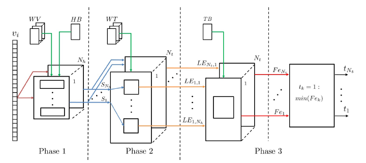Figure 5: Accelerator Architecture

Regarding the implementation of the hardware accelerator, a major consideration involves the arithmetic, fixed or floating-point, that will be used for the calculations. The proposed design uses fixed-point arithmetic for all linear functions (add, mul, cmp) and single-precision floating-point for non-linear functions, like log and exp in (12). To specify the range of the fixed-point arithmetic, simulations were run and statistics were collected based on all available training and test data patterns.

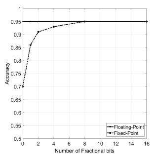Figure 6: Accuracy vs Fractional bits (N_h = 32)

Figure 6 shows the accuracy results for various fixed-point number configurations. It can be seen that by using 16-bits fixed-point numbers, with the first 8 bits being used for the sign bit and the integer part and the remaining 8 bits for the fraction, a good classification accuracy of 95% can be achieved.

The proposed architecture is based on equations (11), (12) and (14) and is organized into three separate phases, shown in Figure 5. The time required to execute each phase determines the performance increase that can be achieved by proper pipeline. Whenever needed, the results of each phase are stored in shared memories and/or cascaded registers. The weights and biases are stored in dual-port RAMs and/or FIFOs, so that they are initialized/updated during system operation when new training data have been used.

A detailed description of the three phases comprising the accelerator architecture follows:

• Phase 1: Each image consists of a set of pixels, which are represented as binary values. This simplifies the multiplication part of (11), since instead of arithmetic multiplications, low complexity multiplexing functions can be used. The incoming image determines the weights that have to be used in the sum of products. Figure 7 shows a detailed scheduling of the operations implemented in this phase. Each load operation refers to reading WV values from memory. The sel of each multiplexer is connected to the corresponding pixel of the input image. This module needs 2 clocks to perform load and mux operations in order to feed the adder trees. After this point all additions are completed in 6 clocks. A total of 4 such modules is used.

Each of these modules includes 256 adders and is responsible for calculating 8 S_m results. Equation (11) determines that a total of 32 S_m results is needed. Every module operates in a pipeline manner. Although each S_m needs 8 clocks to be calculated, by using pipeline a total latency of 37 clocks is achieved.

Phase 2: Apart from the first addition, phase 2 is implemented using floating-point arithmetic. It was designed using the functionalities of Xilinx’s Floating-point IP core [23]. The architecture of phase 2 and the respective timing diagram is given in Figure 8. Equation (12) is implemented in two similar and with same latency stages: exp(a + b) and ln(a + b).

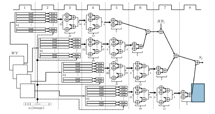Figure 7: Phase 1 of Accelerator Architecture: Addition and Multiplexing Scheduling

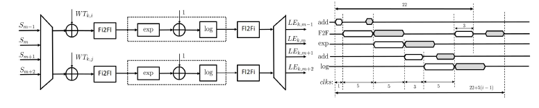Figure 8: Phase 2 of Accelerator Architecture: Block Design (left) and Timing Diagram (right)

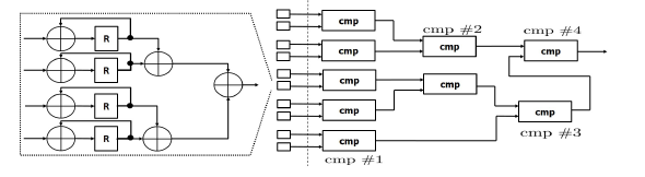Figure 9: Phase 3 of Accelerator Architecture: Block Design

 

Therefore, two LE values can be calculated simultaneously using pipeline. For optimum performance, multiplexing of the incoming S_m values is performed, thus reducing the hardware complexity without decreasing the processing rate, and then fixed-to-floating point transformation is applied. Since the Fixed-point addition with the Fixed-to-Floating (F2F) operation lasts for less than the duration of each of the aforementioned processing stages, the same floating-point circuit (indicated with a dotted line) can be used for processing continuously a stream of S_m values. Since a total of N_hxN_t LE values have to be calculated, the number of such circuits is determined by the multiplexing/demultiplexing used. Fl2Fi in this figure corresponds to floating-to-fixed transformation. Phase 2 is the slowest phase of the whole accelerator. Reducing its latency would lead to improvement of the whole processing rate of the accelerator. To achieve this, sets of four LE values are calculated simultaneously. However, the required DSP resources are doubled.

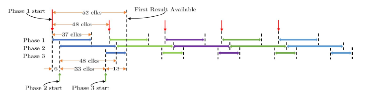Figure 10: Pipeline strategy applied between processing phases

• Phase 3: The last phase is divided into two distinct sub-phases. The first accumulates the LE_k,j inputs from Phase 2 to produce the Fe_k results (13). The second sub-phase uses the N_t computed Fe values in parallel and in a few clock cycles determines the digit (14) that corresponds to the class of the input image. Figure 9 presents the architecture of Phase 3.

Since all these phases have different processing times and do not require all the results of the previous phase to be available in order to proceed, pipeline can be used for increasing the whole system’s processing rate. The latency of phase 1 is 37 clocks. In phase 2 the latency is 48 clocks and 10 such circuits are used in parallel. The combined latency for phase 3 is 10 clocks and 10 circuits implementing the accumulation process are used. Therefore the total latency per hNN without pipeline is 95 clock cycles. A pipeline of two is used and so the module is ready to receive new images every 48 clock cycles, with a latency of 52 clock cycles, as shown in Figure 10.

7. System Prototyping and Performance Results

The above described HDR Cloud Service has been implemented and tested in Xeon and Power8 servers (Table 1) while the hardware accelerator has been implemented in a Virtex-7 FPGA. For generating various workloads, an i7 server has been used, where various clients were implemented with user-defined workload patterns. The HDR clients send bunches of images over 1 Gbps ethernet link.

7.1. Software only Configuration

The applications of clients and servers were developed in C. Provided that HDR servers are multi-threaded, a very popular API is used for threading an application, known as POSIX Thread [24]. Also, CBLAS library is used for performing all the necessary vector and matrix operations. The OS of all platforms is Linux ubuntu 15.10. In order to validate the efficiency of this configuration, the data rate achieved (in KImages/secs) for various computing servers (Table 1) and for various bunches of images (KImages/req) was measured. To preserve consistency with the hardware implementation, the number of hidden nodes used in sNNs is 32.

Table 1: Clients and Server Platforms

Platfrom	CPU			Memory
	Cores	GHz	GB	Type	MHz
Xeon	6	1.60	16	DDR3	2133
Power8	4	3.00	64	DDR4	1600/1333
Power8	8	3.32	64	DDR4	1600/1333

When the number of images per request is small the total performance drops because the time between consecutive requests is much higher compared to the processing time of each request. On the other hand, the number of images per request does not affect the performance when it is more than a few hundreds since the overhead is absorbed. This can be seen in Tables 2 and 3.

Table 2: Processing rate [KImgs/sec] using software HDR implementation (N_t =32 and 1KImgs/req)

	Number of HDR Clients
Servers	1	4	16	64
Intel Xeon	13.20	55.01	82.31	83.10
Power8	16.12	50.52	95.01	98.14
Power8	14.39	46.92	149.03	171.86

Table 3: Processing rate [KImgs/sec] using software HDR implementation (N_t =32 and 10KImgs/req)

	Number of HDR Clients
Servers	1	4	16	64
Intel Xeon	13.31	55.36	82.11	82.77
Power8	16.20	59.82	98.13	100.09
Power8	14.48	54.88	155.33	171.20

Based on Tables 2 and 3, it is evident that the system performance has a linear relation with the number of HDR clients. For a small number of clients, the system is not fully utilized due to the communication overhead. Each client waits for the completion of a request before sending a new one. As the number of clients increases, this overhead is amortized and full system utilization is achieved. So, the performance increases with the increase in the number of clients. The performance reaches different maximum values, depending on the server platform used. This is mainly due to the fact that each server has different number of CPU cores (Table 1). As mentioned, when multiple threads are running, they are distributed to different cores and exploit better the capabilities of each CPU.

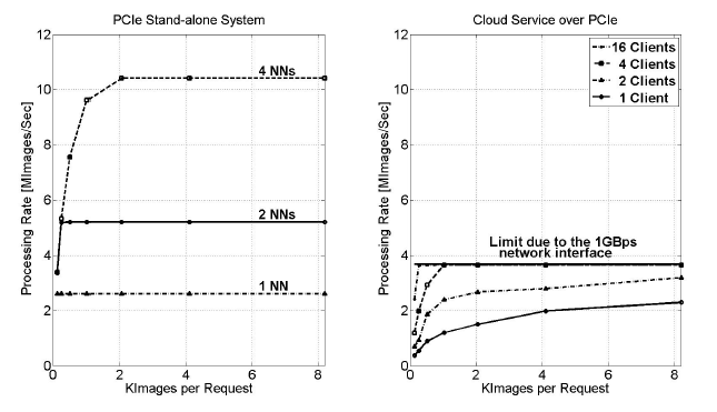Figure 11: Processing rate using hardware HDR implementation over PCIe

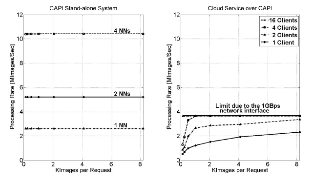Figure 12: Processing rate using hardware HDR implementation over CAPI

7.2. Hardware only Configuration

As far as the accelerator is concerned, based on the latency numbers provided above, a processing rate of 2.6 MImages/sec, at 125 MHz, is achieved by each hNN module. To maximize the total accelerator performance, four hNN modules operate in parallel. That results to a total processing rate of

10.4 MImages/sec, at 125 MHz. The limitation of four modules is introduced by the available resources of the specific Virtex-7 FPGA board (Table 4).

The accelerator supports two interfaces, PCIe Gen

3.0 with 8 lanes and Coherent Accelerator Processor Interface (CAPI). In both cases, a databus of 1024 bits is used that provides images up to four hNNs simultaneously.

The accelerator was attached to a Power8 server with 8 cores (Table 1). For each interface (PCIe, CAPI) two different sets of experiments were conducted in order to measure the performance of the hardware configuration. The results concerning the PCIe are shown in Figure 11. The left part illustrates the accelerator’s processing rate by varying the number of images per request as well as the number of hNNs implemented in the accelerator. In this case, the images are stored locally to the server and not received from multiple clients over the network. The number of images per request does not affect the performance when 1 or 2 hNNs are implemented in the accelerator. The rate is 2.6 MImages/sec and 5.2 MImages/sec correspondingly. When 4 hNNs are integrated, the maximum rate (10.4 MImages/sec) is achieved when each request contains at least 2K images.

Table 4: Implementation parameters of a neural network (N_t =32, XC7VX690T-2 Virtex-7 FPGA)

	Phase 1	Phase 2	Phases 3-4	Total
BRAMs	4 %	1 %	1 %	6 %
DSP	–	13 %	–	13 %
FFs	1 %	3 %	1 %	5 %
LUTs	7 %	8 %	1 %	16 %
Slices	–	–	–	18 %

The right part of Figure 11 illustrates the processing rate, when 4 hNNs operate in parallel, varying the number of connected clients over the network. It is obvious that the maximum rate of this set-up can be achieved even for a small number of active clients. Although in the case of 4 hNNs the maximum achievable rate is 10.4 MImages/sec it can be seen that the maximum processing rate of the whole set-up is less due to the used network interface (934.4 Mbps data rate over a 1 Gbps Ethernet link), since the communication interface becomes the systems bottleneck. Nevertheless, the system with 1 Gbps network interface and hardware acceleration is up to 21 times faster compared to the software implementation.

The achieved processing rates when CAPI is used are shown in Figure 12. The performance is slightly better when 4 hNNs are implemented in the accelerator as it can be seen in the left part of the figure. In this case, the accelerator reaches its maximum value even for a small number of images per request. So, the configuration with CAPI outperforms the configuration with native PCIe. Traditional I/O attachment protocols, like PCIe, introduce significant device driver and operating system latencies, since an application calls the device driver to access the accelerator and the device driver performs a memory mapping operation. With CAPI instead, the accelerator is attached as a coherent CPU peer over the I/O physical interface.

8. Conclusions

The design and implementation of a computing engine for handwritten digits recognition was presented. This engine can be used for cloud applications and achieves high performance, in terms of processing rate, when a hardware accelerator with multiple neural networks is used, as demonstrated by experimental results. Details of neural networks implementation on reprogrammable logic have also been described. The architecture can be parameterized in order to achieve the best compromise between hardware complexity and processing performance.

1. Smola and S. VishwanathanKevin, Introduction to Machine Learning. Cambridge, UK: Cambridge University Press, 2008.
2. Fischer and C. Igel, “An introduction to restricted boltzmann machines.,” in CIARP (L. Alvarez, M. Mejail, L. G. Deniz, and J. C. Jacobo, eds.), vol. 7441 of Lecture Notes in Computer Science, pp. 14–36, Springer, 2012.
3. Fischer and C. Igel, “Training restricted Boltzmann machines,” Pattern Recogn., vol. 47, pp. 25–39, Jan. 2014.
4. Bougioukou, N. Toulgaridis, and T. Antonakopoulos, “Cloud services using hardware accelerators: The case of handwritten digits recognition,” in Proceedings of the 6th International Conference on Modern Circuits and Systems Technologies (MOCAST), (Thessaloniki), 4-6 May 2017.
5. Toulgaridis, E. Bougioukou, and T. Antonakopoulos, “Architecture and implementation of a restricted Boltzmann machine for handwritten digit recognition,” in Proceedings of the 6th International Conference on Modern Circuits and Systems Technologies (MOCAST), (Thessaloniki), 4-6 May 2017.
6. LeCun, C. Cortes, and C. Burges, “MNIST handwritten digit database,” 2010. http://yann.lecun.com/exdb/mnist/.
7. C. Cires¸an, U. Meier, J. Masci, L. M. Gambardella, and J. Schmidhuber, “Flexible, high performance convolutional neural networks for image classification,” in Proceedings of the Twenty-Second International Joint Conference on Artificial Intelligence – Volume Volume Two, IJCAI’11, pp. 1237–1242, 2011.
8. Ciresan, U. Meier, and J. Schmidhuber, “Multi-column deep neural networks for image classification,” in Proceedings of the 25th IEEE Conference on Computer Vision and Pattern Recognition (CVPR 2012, pp. 3642–3649, 2012.
9. -Y. Lee, P. W. Gallagher, and Z. Tu, “Generalizing pooling functions in convolutional neural networks: Mixed, gated, and tree,” ArXiv e-prints, Sept. 2015.
10. Wan, M. Zeiler, S. Zhang, Y. LeCun, and R. Fergus, “Regularization of neural networks using dropconnect,” in Proceedings of the 30th International Conference on International Conference on Machine Learning – Volume 28, ICML’13, 2013.
11. Benenson, “Classification datasets results.” https: //rodrigob.github.io/are_we_there_yet/build/ classification_datasets_results.html.
12. -j. Zhang and N.-f. Xiao, “Parallel implementation of multilayered neural networks based on map-reduce on cloud computing clusters,” 02 2015.
13. Teerapittayanon, B. McDanel, and H. T. Kung, “Distributed deep neural networks over the cloud, the edge and end devices,” 09 2017.
14. L. Ly and P. Chow, “A high-performance fpga architecture for restricted boltzmann machines,” in Proceedings of the ACM/SIGDA International Symposium on Field Programmable Gate Arrays, FPGA ’09, (New York, NY, USA), pp. 73–82, ACM, 2009.
15. K. Kim, L. C. Mcafee, P. L. Mcmahon, and K. Olukotun, “A highly scalable restricted boltzmann machine fpga implementation,” in Proceedings of the International Conference on Field Programmable Logic and Applications, pp. 367–372, 08 2009.
16. Larochelle and Y. Bengio, “Classification using discriminative restricted boltzmann machines,” in Proceedings of the 25th International Conference on Machine Learning – ICML ’08, (Helsinki, Finland), pp. 536–543, 2008.
17. Larochelle, M. Mandel, R. Pascanu, and Y. Bengio, “Learning algorithms for the classification restricted boltzmann machine,” J. Mach. Learn. Res., vol. 13, pp. 643–669, Mar. 2012.
18. Hinton, “Training products of experts by minimizing contrastive divergence,” Neural Computation, vol. 14, p. 2002, 2000.
19. J. Donahoo and K. L. Calvert, TCP/IP Sockets in C: Practical Guide for Programmers. San Francisco, CA, USA: Morgan Kaufmann Publishers Inc., 2nd ed., 2009.
20. PCI SIG, PCI Express Base Specification, Revision 2.1, March 2009.
21. IBM Systems Magazine, A Deeper Look at POWER8 CAPI and Data Engine for NoSQL, May 2015. http: //ibmsystemsmag.com/power/businessstrategy/ competitiveadvantage/capi-deep-look/.
22. LeCun, S. Chopra, R. Hadsell, M. Ranzato, and F. Huang, “A tutorial on energy-based learning,” in Predicting Structured Data (G. Bakir, T. Hofman, B. Sch¨olkopf, A. Smola, and B. Taskar, eds.), MIT Press, 2006.
23. Xilinx Inc., Floating-Point Operator. https://www.xilinx. com/products/intellectual-property/floating_pt. html.
24. Nichols, D. Buttlar, and J. P. Farrell, Pthreads Programming. Sebastopol, CA, USA: O’Reilly & Associates, Inc., 1996.

(Click to view)

(Click to view)