1. Introduction

Proton Exchange Membrane Fuel Cells are complex multi-physics systems (chemical, electrical, fluidic, thermal, and mechanical phenomena are inter-acting with one another). This makes the modeling and fault diagnosis of PEMFC systems a very difficult task. Furthermore, when the modeling is based on experimental testing and experimental data, some limitations are usually faced. For example, many physical system data may be absent or difficult to obtain with the system’s supplied data acquisition. Furthermore, due to warranty issues, the addition of sensors might be difficult since only limited access to the systems is allowed. Likewise, other specific parameters might be unobtainable due to manufacturer confidentiality issues.

This paper is an extension of work originally presented in the 7^th International Conference on Modeling, Simulation, and Applied Optimization (ICMSAO) [1]. It presents a novel approach, in which the Siemens software, LMS AMESim 14, is used as an alternative modeling tool to model a PEMFC system when such limitations are faced. The LMS AMESim software can serve as an excellent and attractive simulation and modeling platform for different complex physical systems such as automobile and aviation systems as well as power generation systems and transmission lines. Moreover, it has outstanding simulation capabilities that makes it an excellent platform for fault simulation, and fault diagnosis studies. The graphical user interface comprehensive library it contains makes it very easy to compile a complete system model from different system components. Instead of writing all the modeling equations which could be time consuming and is prone to modeling errors, a user can use a ready accurate model better and focus on the parameter identification step in order to find the model that matches the pursued system performance measures. Furthermore, a researcher can easily change the scripts of the components used to better suit their system’s design, as well as create new libraries with more specific components.

The ElectraGen^TM 3 kW PEMFC system shown in Figure 1, is an actual commercial system used in practice in many sectors, especially in telecommunication companies. It uses hydrogen gas supplied from pressurized hydrogen cylinders as the anode fuel, and atmospheric air supplied by a compressor and humidified through a built-in humidity exchanger as the cathode fuel. The ElectraGen^TM system is an outdoor air cooled system, and it is only operable at ambient temperatures ranging from –40°C to 50°C. It contains a total of 38 cells and can produce up to 3 kW of unregulated DC output power and has a rated voltage of 48V.

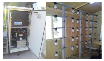Figure 1: The ElectraGen^TM PEMFC system and the 3 kW Load.

The module contains the ElectraGen^TM 3 kW Fuel Cell stack with integrated microprocessor controller and safety features, a hydrogen pressure gauge which gives an indication of fuel level and the 3kW load which consists of 30 lamps, 100W each (see Figure 1). The system is connected through data acquisition to a GUI based on LabVIEW to monitor and log the different system variables (stack current, stack voltage, external voltage, individual cell voltages, cabinet temperature, cathode air temperature, coolant temperature, exhaust temperature, and hydrogen pressure). The ElectraGen^TM system is installed outdoor and the experimental data sets collected from the system were taken at extreme environmental conditions in the summer at noon with the ambient temperature ranging from 48°C to 52°C. However, due to warranty issues, limited access to the systems was allowed and limited data was obtainable from the data acquisitions. Moreover, due to confidentiality issues with the manufacturer, several physical parameters were unobtainable such as active cell area, membrane length, volumes of cathode and anode chambers, mass of stack, etc. This made it very difficult to model the system and develop an accurate fault diagnosis scheme. Therefore LMS AMESim was used as an alternative modeling platform since all the common PEMFC modeling equations available in literature [2, 3] are already embedded in its library components.

Furthermore, it is convenient to mention here that the simulated model will not be an exact match for the ElectraGen^TM system since not enough system readings were available to match the model to. However, it is the aim of this work to develop an AMESim model that is as realistic as possible by matching all the known features of the actual physical system (the ElectraGen^TM system) to their equivalents in the AMESim model as best as possible. This model can then be used in the fault diagnosis study.

Section 2 presents the ElectraGen^TM modeling and validation results using the Siemens LMS AMESim Software. In section 3, the simulation of five different system faults is presented, and in section 4 two residual generation techniques are evaluated and then outperforming technique is used to develop a fault diagnosis scheme in AMESim for the ElectraGen^TM system. The fault diagnosis scheme is then evaluated and concluding remarks are finally given in section 5.

2. AMESim Modeling of the ElectraGen^TM 3 kW System

The LMS AMESim software contains several embedded parameter identification tools including Genetic Algorithms (GA). However, in order to be able to use such tools efficiently, several software licenses are needed.  To further explain this, GA is a population based mechanism that is known to be successful because it performs parallel evaluations, and when only one AMESim license is available, using GA becomes impractical. As an example, if the GA has 20 individuals in its population, and with a preset maximum number of generations of 500, this is equivalent to 10,000 runs of the software. With one system license, the software will be unable to perform parallel evaluations. Thus, if a single run of the software takes 1 minute, then the parameter identification process using GA and one system license will take 10,000 minutes (almost seven days).

As a result, matching the parameters of the AMESim model to the actual system performance of the ElectraGen^TM system was done through trial and error.  The LMS AMESim model developed for the ElectraGen^TM PEMFC system is presented in Figure 2.

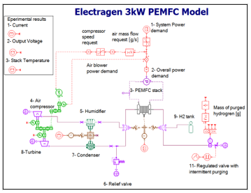Figure 2: ElectraGen^TM 3 kW system’s model in AMESim.

2.1.  AMESim Model Parameter Identification

The actual power demand data collected experimentally from the ElectraGen^TM system was used as the input to the system in Figure 2.  After several trial and error attempts to match the stack voltage, stack current, and stack temperature values as best as possible to the actual experimental data collected from the system; the best obtained match is depicted in the following figures: Figure 3 gives the power demand input of the modeling data set, and Figures 4, 5 and 6 presents a comparison between the actual experimental current, stack voltage and stack temperature respectively to those resulting from the AMESim simulation model.

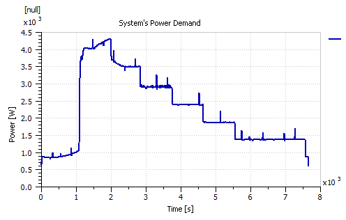Figure 3: Power demand of the AMESim modeling data set.

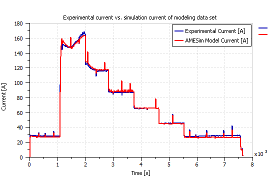Figure 4: Experimental versus AMESim model’s resulting current of the modeling data set.

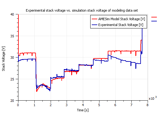Figure 5: Experimental versus AMESim model’s resulting stack voltage of the modeling data set.

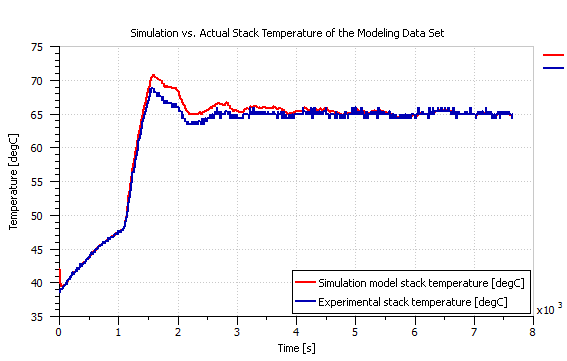Figure 6: Experimental versus AMESim model’s resulting stack temperature of the modeling data set.

2.2.  AMESim Model Validation

Two other ElectraGen^TM experimental data sets were used to validate the obtained AMESim model of Figure 2. Figure 7 presents the power demand of the first validation example and Figures 8 and 9 compare the actual experimental current and stack voltage to those obtained from the LMS AMESim model respectively. Similarly, the power demand of the second validation example is given in Figure 10, and a comparison between the actual and simulation current is presented in Figure 11, whereas a comparison between the actual and simulation stack voltage is presented in Figure 12.

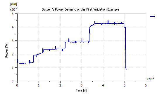Figure 7: Power demand of the first validation example.

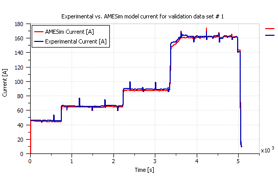Figure 8: Actual versus simulation current of the first validation example.

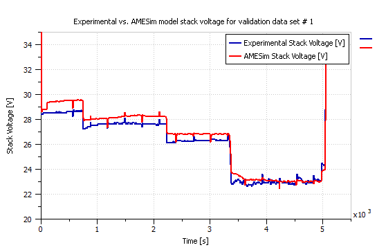Figure 9: Actual versus simulation stack voltage of the first validation example.

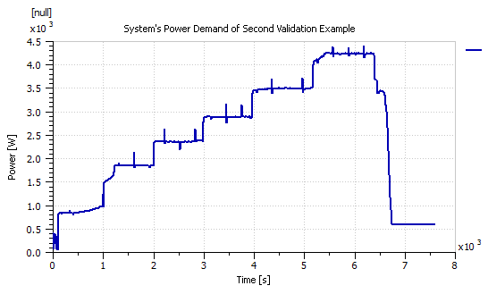Figure 10: Power demand of the second validation example.

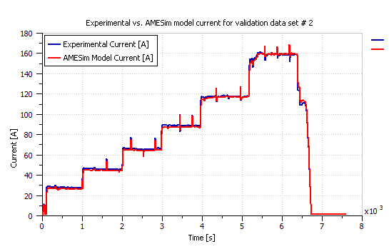Figure 11: Actual versus simulation current of the second validation example.

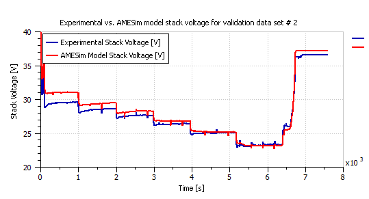Figure 12: Actual versus simulation stack voltage of the second validation example.

Obviously, a perfect representation of the ElectraGen^TM system is unobtainable through trial and error alone.  Nevertheless, after validation, the AMESim obtained model proved to give a proper representation of the system’s performance and was therefore used in the following fault diagnosis study.

Moreover, if resources (multiple licenses of the software) were available, a much more accurate representation of the system would have been achievable through the use of Genetic Algorithms in the parameter identification approach in AMESim, which would have in turn lead to a better fault diagnosis study.

3. Fault Simulation Using AMESim Model

Several faults were induced in the AMESim model and the system’s performance measures towards those faults were recorded. The induced faults are:

1. Drying
2. Flooding
3. Air leakage
4. Hydrogen Leakage
5. Cooling System Failure

The above faults were simulated using different techniques.

3.1.  Drying

Zawodzinski et al. were the first to describe the water content in the membrane by (λ) in [4] in order to estimate its state of humidity. As presented in (1), λ represents the ratio between the number of water molecules in the membrane to the number of ( ) charge sites in the Nafion layer of the membrane [5].

The AMESim PEMFC stack module automatically calculates the water content λ in the membrane. Therefore, when simulating drying or flooding, λ would give an indication towards the membrane’s state of health.

However, λ cannot be used in the fault diagnosis study because this parameter is not readily available in commercial fuel cells. Furthermore, the PEMFC undergoes drying condition when the water content in the membrane λ drops below 4 [6].

Therefore in order to simulate drying, the humidity level of the input air was set to be 0% and the target humidity level of the humidifier was dropped to 10% only. The water content in a healthy stack and that of a drying stack are compared in Figure 13. The water content of the stack that is undergoing drying is obviously well below 4.  Figure 14 on the other hand depicts the difference between the polarization curve of a healthy stack and a drying stack. It is noticed that drying results in a significant voltage.

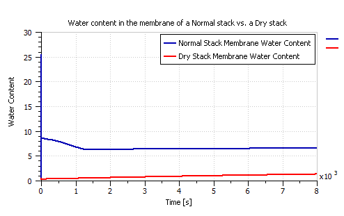Figure 13: The water content in the membrane (λ) of a normal stack versus a dry stack.

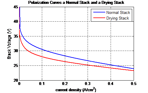Figure 14: Normal stack’s polarization curve in comparison to a dry stack’s polarization curve.

3.2.  Flooding

Flooding was simulated by dropping the stack temperature to 25°C while increasing the humidifier’s target humidity level to 100%. Flooding affected both the voltage and current profiles of the stack as depicted in the polarization curve comparison given in Figure 15. Furthermore, Figure 16 shows the water content λ of the simulated flooded stack.

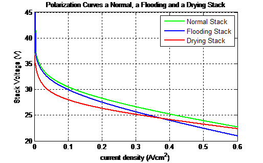Figure 15: Comparison of pressure drop in a normal stack, a flooding stack and a drying stack.

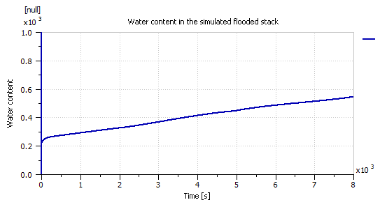Figure 16: The water content in the membrane (λ) of the simulated flooding stack

Note that both flooding and drying result in similar effects to the stack’s polarization curve. However, flooding seemed to also cause a distinctive effect on the cathode pressure drop. As the stack gets flooded with water, the pressure drop across the cathode increases.  Nonetheless, in order to clearly see this effect on cathode pressure, the stack had to be fed with a step power demand profile such as that of Figure 17.  The cathode pressure of both the healthy and flooded stacks with respect to the power demand input of Figure 16 are compared in Figure 17. The flooded stack showed a steeper drop in pressure when compared to the healthy stack.

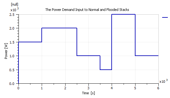Figure 17: Power demand input to normal stack and flooding stacks.

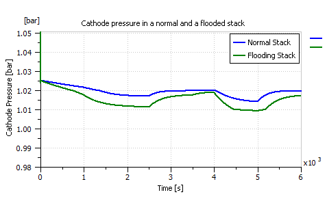Figure 18: Comparison of pressure drop in a normal stack and a flooding stack.

3.3.  Air leakage

In order to simulate air leakage, a relief valve was added right after the humidifier as depicted in Figure 19, and was set to leak air at a rate of around 10 g/s. Figure 20 shows the amount of leakage introduced in g/s. Furthermore, Figure 21 compares the input air flow rate to the PEMFC stack with and without air leakage.

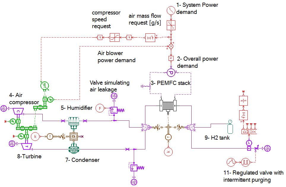Figure 19: The relief valve added to the AMESim model to simulate air leakage.

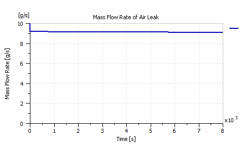Figure 20: The flow rate of the air leakage induced to the PEMFC system.

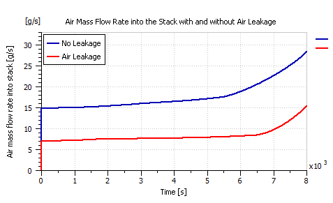Figure 21: Input air flow rate to the stack with and without air leakage.

It can be deduced from the polarization curve comparison depicted in Figure 22 that the air leakage had no noticeable effect on the stack’s current or voltage. However, it was noticed to impose a significant effect on the cathode pressure. To better see this effect, both the healthy and air leaking stacks were fed with the step power demand of Figure 17. Figure 23 shows the air leakage effect on the cathode pressure drop when compared to a non-leaking stack.

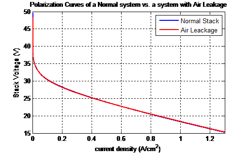Figure 22: Polarization curves of a normal system vs. a system undergoing air leakage.

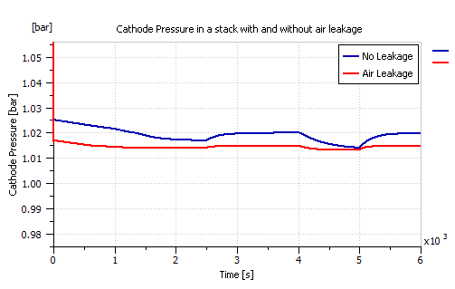Figure 23: Pressure drop in the cathode of a normal system vs. a system undergoing air leakage.

3.4.  Hydrogen leakage

Similar to air leakage, hydrogen leakage was also simulated through the addition of a relief valve right after the hydrogen canister as depicted in Figure 24 in order to leak hydrogen at a rate of 10 g/s.  Figure 25 shows the amount of hydrogen leakage introduced in g/s.

Hydrogen leakage was found to result in a slight effect on stack’s polarization curve as shown in the comparison of Figure 26. Furthermore, hydrogen leakage was also found to affect the anode pressure as shown in Figure 27, but had no significant effect on the cathode pressure as seen in Figure 28.

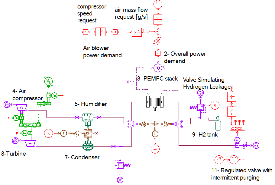Figure 24: The relief valve added to the AMESim model to simulate Hydrogen leakage.

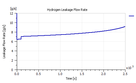Figure 25: The flow rate of the Hydrogen leakage induced to the PEMFC system.

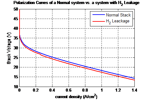Figure 26: Polarization curves of a normal system vs. a system undergoing Hydrogen leakage.

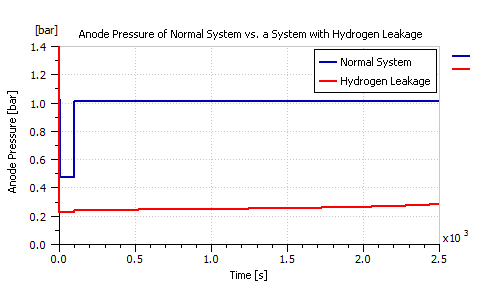Figure 27: Anode pressure of a normal system vs. a system undergoing Hydrogen leakage.

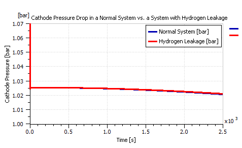Figure 28: Pressure drop in the cathode of a normal system vs. a system undergoing Hydrogen leakage.

3.5.  Cooling Failure

The stack temperature of the ElectraGen^TM system should be maintained at a temperature value between 60°C to 65°C for maximum efficiency through air cooling. However, it is also convenient to mention that the stack temperature should never reach any value above 75°C in order to avoid damage of the membrane. Thus, it is important to flag a cooling system failure as soon as the stack temperature reaches 75°C or higher. Hence, the stack’s temperature was increased to 75°C in order to simulate cooling failure. The polarization curve was found to undergo a significant effect with the increase in stack temperature as shown in Figure 29.

Note that the 75°C stack temperature results in a slight improvement in the system’s polarization curve because the resistive components in the activation and ohmic voltage drop will decrease with the increase in stack temperature. However, at such an elevated temperature, drying of the stack will be inevitable. Furthermore, comprehensive literature review [7] revealed that operating the PEMFC at higher stack temperatures is a common stressor for almost all health degradation mechanisms. Thus, this slight improvement in the polarization curve is worthless since it will significantly shorten the PEMFCs lifespan.

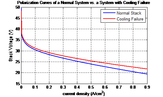Figure 29: Polarization curve of a normal system vs. a system undergoing cooling failure.

Nonetheless, the stack temperature should be the main parameter used to detect the presence of cooling failure regardless of the effects on the voltage and current profiles. As soon the stack’s temperature reading reaches 75°C is a cooling system failure fault should be flagged.

Note from Figure 29 that there is an improvement in the voltage performance of the fuel cell with the increase of stack temperature. This is expected since the rate of chemical reactions increase with the temperature causing this increase in voltage. However, it should also be noted that at this temperature value of 75°C, drying of the membrane is inevitable. Furthermore, high stack temperature is a well-known stressor for PEMFCs [8 – 11]. Thus, operating the system at such elevated stack temperatures will significantly reduce its lifespan, which makes this small voltage improvement at high stack temperature values worthless.

4. Fault Diagnosis

In this work, the model based fault diagnosis approach is based on the real-time comparison between the actual system performance and the performance predicted by the developed AMESim model. Any predicted discrepancies will be analyzed to determine the type of system fault occurring at the moment.

4.1.  Residual generation

It can be concluded from the previous section that in order to detect discrepancies between the actual system and its developed model that can help in the fault detection and isolation process, five residuals (see Figure 30) should be generated based on the following five system variables: stack voltage (V_stack), current (I), stack temperature (T_stack), cathode pressure (P_Cathode) and anode pressure (P_anode).

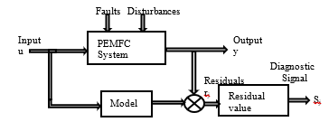Figure 30: Residual generation diagram [12].

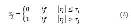
Several forms exist in literature for the calculation of residuals. In the simplest form given in (2), the absolute value of the residual (r_j) is compared to a relative threshold value (τ_j). The diagnostic signal (S_j) is then set to be “0” if the absolute residual is less than or equal to the threshold to indicate that no discrepancy is detected, and “1” if the absolute residual is greater than the set threshold which indicates that a discrepancy is detected [12]

          Note that basing the fault diagnosis approach on the residuals calculated in (2) makes the approach prone to diagnosis errors. This is because the residuals of (2) are highly sensitive to instantaneous changes in the system such as the electromagnetic disturbance pulses which act on the system’s measured signals as well as the occurrence of actual system faults.

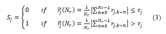
Therefore, the calculation of those residuals can be slightly altered to decrease their sensitivity to disturbances. Thus, instead of calculating instantaneous residuals, they can be calculated over a moving window of time and judging the average of all residuals in that window as explained by (3), where N_r represents the number of residuals in the window [13]:

The threshold value for each residual is given in Table 1, and it was set based on the accuracy of the actual system sensors installed in the ElectraGen^TM PEMFC system.

Table 1: Accuracy of actual sensors used to measure system variables

System variable	Sensor accuracy
Stack Voltage (Vstack)	± 0.5 V
Current (I)	± 1 A
Stack Temperature (Tstack)	± 3 °C
Cathode Pressure (Pcathode)	± 1 mbar
Anode Pressure (Panode)	± 1 mbar

4.2.  Sensitivity assessment

Both the residual calculation techniques of (2) and (3) were implemented in LMS AMESim to study and assess their effectiveness and test their sensitivity towards electromagnetic disturbance pulses. Thus, a noisy step power demand signal with disturbance pulses was generated to help with the assessment. The system estimator however was fed with a clean power demand signal to test the diagnostic signals sensitivity toward those disturbance pulses.

The residuals that were calculated by the system are: r₁ which is based on the stack temperature (T_stack), r₂ which is based on the stack voltage (V_stack), r₃ which is based on the current (I), r₄ which is based on the anode pressure (P_anode) and r₅ which is based on the cathode pressure (P_cathode). On the other hand, S_i is the respective diagnostic signal r_i.

The faults being detected by the proposed fault diagnosis approach are: (f₁ = Drying, f₂ = Flooding, f₃ = Air Leakage, f₄ = Hydrogen Leakage, and f₅ = Cooling Failure). The results of section III are summarized in Table 2 to help in the fault discrimination process, where 0 indicates that no discrepancies are detected between the predicted value and the actual measured value, and 1 indicates the positive detection of discrepancies whereas X indicates the fault exists whether the diagnostic signal detects discrepancies in the system variable or not. Note that the cooling failure that f₅, is set to be flagged as soon as the stack temperature reaches a value of 75°C (i.e. based on S₁) regardless of the effects on the stack voltage and current (i.e. S₂ and S₃).

Table 2: The effect of faults on diagnostic signals

fault	S1	S2	S3	S4	S5
f1	0	1	1	0	0
f2	0	1	1	0	1
f3	0	0	0	0	1
f4	0	1	1	1	0
f5	1	X	X	0	0

Figure 31 shows the fault diagnosis system built based on the instantaneous diagnostic signals calculation of (2). Figure 32 shows the noisy power demand signal fed to the actual system being diagnosed and the clean power demand signal fed to the system estimator.  The diagnostic signals calculated based on the instantaneous residuals of (2) are shown in Figure 33.

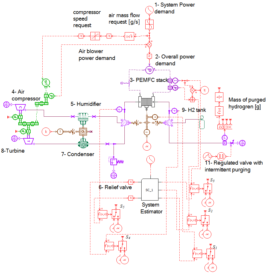Figure 31: Fault diagnosis system based on instantaneous diagnostic signals.

It is obvious from Figure 33 that the diagnosis approach based on the instantaneous residuals in (2) is impractical and highly sensitive to electromagnetic disturbance pulses, which can therefore result in the detection of a faults when no fault actually exists. For instance, at around 150 s, both S₂ and S₃ diagnostic signals were triggered, which from Table 2 , will indicate the presence of the first fault f₁ (Drying).

Afterwards, the diagnostic signal of (3) was also implemented in LMS AMESim in order to be assessed based on three different moving windows of time (5 s, 10 s and 15 s). The same power signals of Figure 32 were used in the assessment to evaluate its sensitivity towards electromagnetic disturbance pulses. The fault diagnosis system built based on the diagnostic signals calculation of (3) is presented in Figure 34.

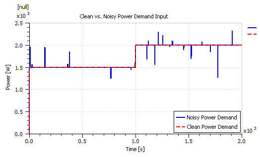Figure 32: Clean and noisy power demand signals.

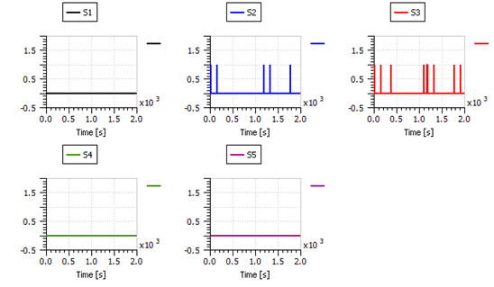Figure 33: The effect of the pulsating noise on the five diagnostic signals.

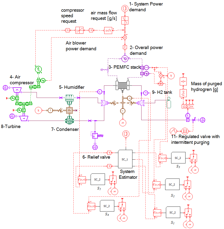Figure 34: Fault diagnosis system based on diagnostic signals calculated over a window of time.

Note that a super-component was added to this model to help calculate the diagnostic signal over three different windows of time equal to 5 s, 10 s and 15 s. The contents of this super-component for the 5 s moving window of time is presented in Figure 35, whereas the super-component for the 10 s moving window of time is presented in Figure 36, and finally the super-component for the 15 s moving window of time is presented in Figure 37.

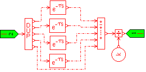Figure 35: Super-component calculating diagnostic signal over a 5 s time window

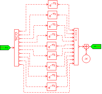Figure 36: Super-component calculating diagnostic signal over a 10 s time window

Furthermore, the effect of the electromagnetic disturbance pulses on the calculation of the five diagnostic signals evaluated using a 5 s moving window of time is presented in Figure 38. Moreover, the effect of the disturbance pulses on the diagnostic signals utilizing a 10 s moving window is presented in Figure 39, and the effect of the disturbance pulses on the diagnostic signals utilizing a 15 s moving window is presented in Figure 40.

Figures 38, 39 and 40 prove that this diagnostic approach of (3) outperforms that of (2). However, it is convenient to mention here that most commercial PEMFC systems commonly have a minimum sampling time of 1 s. Therefore, basing the diagnostic signal on a 5 s window of time can prove to be impractical as seen in Figure 38. Furthermore, the diagnostic signals calculated based on both the 10 s and the 15 s moving windows of time proved to be effective and insensitive to electromagnetic disturbance pulses as seen from Figures 39 and 40. Nevertheless, using a 10 s moving window of time is preferred over the 15 s moving window of time in order to avoid delays in detecting faults as well as saving memory.

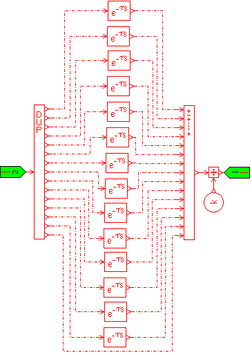Figure 37: Super-component calculating diagnostic signal over a 15 s time window

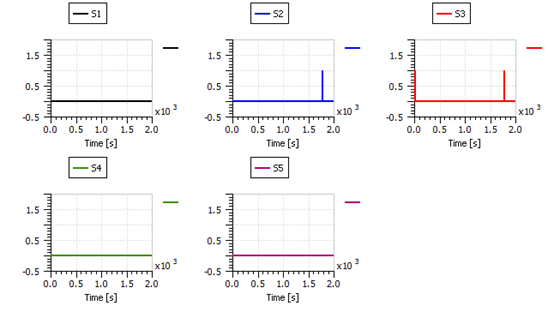Figure 38: The effect of the disturbance pulses on the five diagnostic signals calculated using a 5 s moving window.

Figure 39: The effect of the disturbance pulses on the five diagnostic signals calculated using a 10 s moving window.

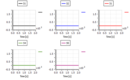Figure 40: The effect of the disturbance pulses on the five diagnostic signals calculated using a 15 s moving window.

4.3.  Fault diagnosis results

To test the proposed fault diagnosis scheme designed using diagnostic signals calculated over a 10 s moving window of time; the five system faults were induced at different times to evaluate the system’s ability to detect and isolate the five system faults.

The first fault to be simulated was membrane drying. Thus, the relative humidity target of the humidifier was dropped to 10% and the effect of this action was immediately captured by the diagnostic signals S₂ and S₃ as seen in Figure 41, which – from Table 2 – clearly indicates the presence fault f₁ (drying of the membrane).

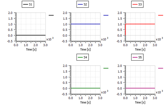Figure 41: The diagnostic signals successfully detecting drying fault.

The second fault to be tested was membrane flooding. Therefore, the relative humidity target of the humidifier was raised to 100% while reducing the stack temperature to 25°C. Again, this action was clearly reflected on the diagnostic signals as seen from Figure 42, and the three diagnostic Signals S₂, S₃ and S₅ were triggered.  However, it was noticed that the effect on the diagnostic signal S₅ was not as fast as that on diagnostic signals S₂ and S₃. This is expected since the increase in pressure drop needs some time to take effect. From Table 2, triggering S₂, S₃ and S₅ at the same time indicates the presence fault f₂ (flooding of the membrane).

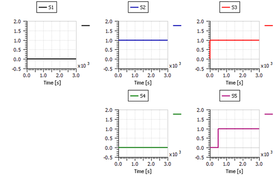Figure 42: The diagnostic signals successfully detecting flooding fault.

          The third fault to be tested was the air leakage in the supply manifold, which was simulated through the addition of a relief valve after the humidifier as shown in Figure 43. This relief valve was set to open with a flow rate of 9 g/s after 500 s of operation. Only one diagnostic signal was affected by this action at around 500 s as depicted in Figure 44. From Table 2, it can be deduced that triggering only S₅ indicates the occurrence of fault f₃ (air leakage).

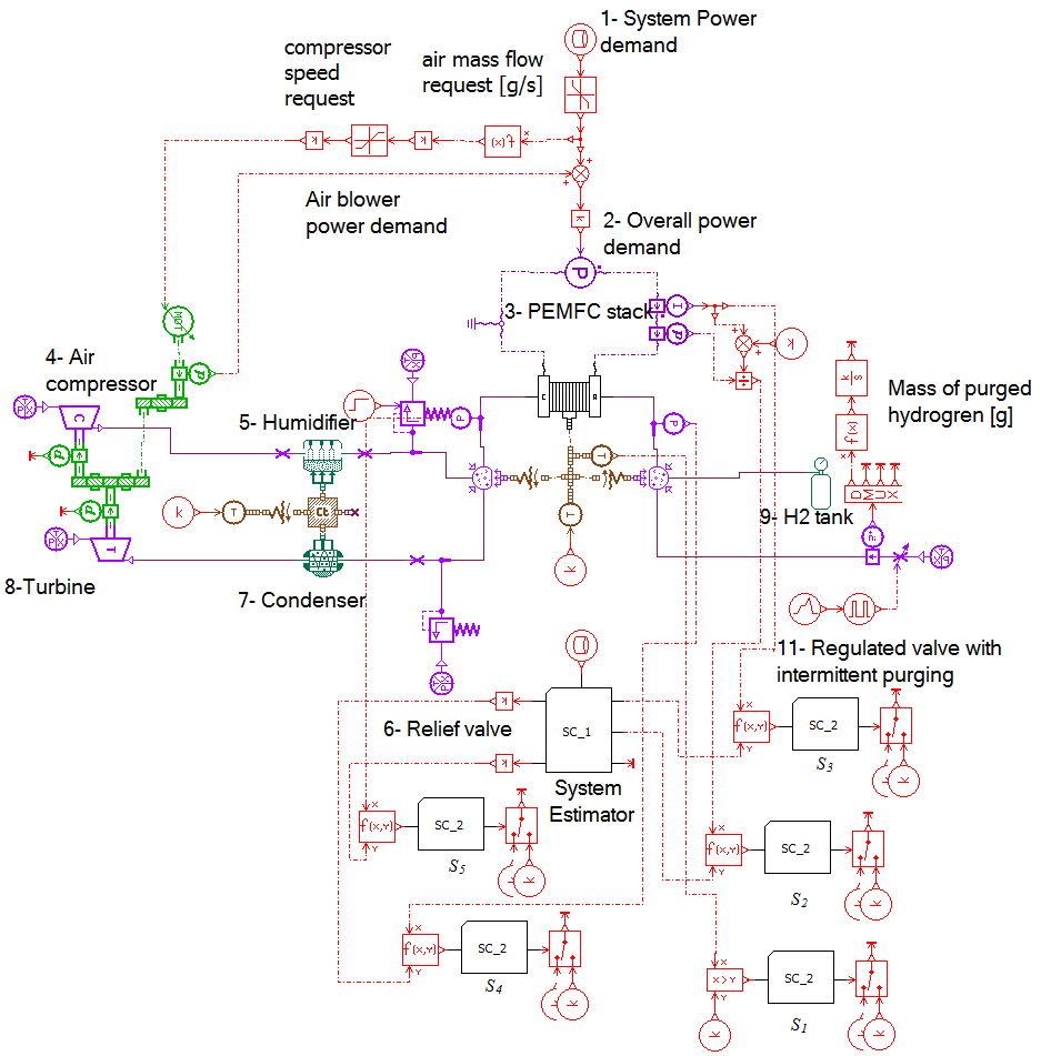Figure 43: The modified diagnosis model with a relief valve to simulate air leakage.

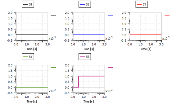Figure 44: The diagnostic signals successfully detecting air leakage fault.

          The next fault to be simulated was hydrogen leakage. As shown in Figure 45, the leakage was simulated through the addition of a relief valve right after the hydrogen supply canister. This valve was set to open with a flow rate of 8 g/s after 500 seconds of operation. The amount of hydrogen leakage can be seen in Figure 46.

From Figure 47, it is noticed that three diagnostic signals were triggered at around 500 s, which are S₂, S₃ and S₄. This clearly indicates the occurrence of fault f₄ (hydrogen leakage) as it can be deduced from Table 2.

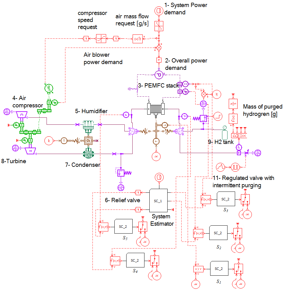Figure 45: The modified diagnosis model with a relief valve to simulate hydrogen leakage.

Finally, the cooling system failure was tested by forcing the stack temperature to rise to 75°C after 1500 s of operation. The three diagnostic signals S₁, S₂ and S₃ were triggered by this action at around 1500 s of operation as shown in Figure 48. As it can be deduced from Table 2, and as previously explained in section III, S₁ alone is enough to flag fault f₅ (cooling failure) regardless of the effects on other diagnostic signals.

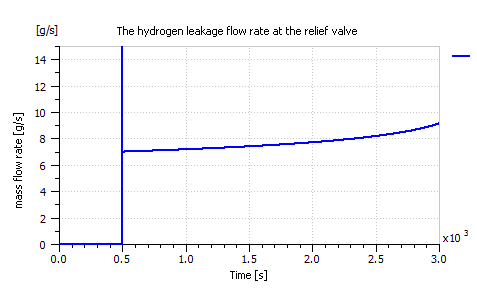Figure 46: The hydrogen leakage flow rate at the relief valve.

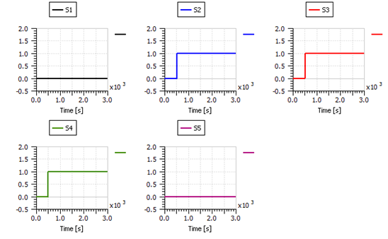Figure 47: The diagnostic signals successfully detecting hydrogen leakage fault

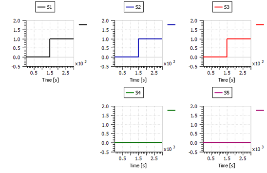Figure 48: The diagnostic signals successfully detecting cooling system failure fault.

5. Conclusion

Fuel cells are extremely attractive clean power generation systems with the capability of someday replacing fossil fuels in the areas of power generation and transportation, while helping clean the environment by significantly lowering the world’s pollution rates. However, to turn this green technology dream into reality, an accurate model that can effectively predict the fuel cell’s performance in different conditions is desired. Such model can then be used to study, simulate, and monitor the behavior of PEMFCs to detect any potential faults that can affect their performance.

Moreover, the complexity of the PEMFC model makes it very difficult and mathematically demanding to try and identify the modeling parameters. Furthermore, other limitations such as the absence of some parameters and confidentiality issues with the manufacturer can also limit the researchers’ ability to develop an accurate fault diagnosis oriented model for a commercial PEMFC system. The Siemens software LMS AMESim 14.2 was used in this work as a solution to overcome such limitations.

A diagnosis oriented model of the ElectraGen^TM PEMFC system was developed in LMS AMESim and five system faults (drying of the membrane, flooding of the membrane, air leakage, hydrogen leakage in the supply manifold, and cooling failure) were simulated to analyze their effect on different system parameters.

Diagnostic signals based on two different residual generation techniques were also assessed in this work, and the outperforming technique was implemented in the proposed diagnosis scheme. This diagnosis scheme was then tested in LMS AMESim against the five system faults under study and it was found to be very successful in both fault detection and discrimination.

Conflict of Interest

The authors declare no conflict of interest.

Acknowledgement

This paper is part of a joint research program funded by United Arab Emirates University (UAEU) and Japan Cooperation Center, Petroleum (JCCP).

1. I. Salim, H. Noura and A. Fardoun, “Fault diagnosis of a commercial PEM fuel cell system using LMS AMESim,” in 7th International Conference on Modeling, Simulation and Applied Optimization, Sharjah, UAE, April, 2017. DOI: 10.1109/ICMSAO.2017.7934890
2. Nehrir and C. Wang, Modeling and Control of Fuel Cells: Distributed Generations Applications, IEEE Press Series on Power Engineering, Wiley, 2009.
3. EG&G Services, Inc., Fuel Cell Handbook, 7th ed., Science Applications International Corporation, DOE, Office of Fossil Energy, National Energy Technology Laboratory, 2004.
4. A. Zawodzinski, M. Neeman, L. O. Sillerud and S. Gottesfeld, “Determination of water diffusion coefficients in perfluorosulfonate ionomeric membranes,” J. Phys. Chem., vol. 95, no. 15, p. 6040–6044, 1991. DOI: 10.1021/j100168a060
5. Springer, T. Zawodzinski and S. Gottesfeld, “Polymer electrolyte fuel cell model,” J. Electrochem. Soc., vol. 138, no. 8, p. 2334–2342, 1991. DOI: 10.1149/1.2085971
6. Khanungkhid and P. Piumsomboon, “200W PEM fuel cell stack with online model-based monitoring system,” Eng. J., vol. 18, no. 4, p. 13 – 26, Oct. 2014. https://doi.org/10.4186/ej.2014.18.4.13
7. I. Salim, H. Noura and A. Fardoun, “A Review on fault diagnosis tools of the proton exchange membrane fuel cell,” 2013 Conference on Control and Fault-Tolerant Systems (SysTol), pp. 686 – 693, Nice, France, Oct. 9-11, 2013. DOI: 10.1109/SysTol.2013.6693877
8. Zhang, C. Song and J. Zhang, “Accelerated lifetime Testing for Proton Exchange Membrane Fuel Cells Using Extremely High Temperature and Unusually High Load,” J. Fuel Cell Sci. Technol., vol. 8, no. 5, p. 051006, 2011. DOI: 10.1115/1.4003977
9. A. Wilkie, J. R.Thomsen and M. L. Mittleman, “Interaction of poly (methyl methacrylate) and nafions,” J. Appl. Polym. Sci., vol. 42, no. 4, p. 901–909, 1991. DOI:10.1002/app.1991.070420404
10. R. Samms, S. Wasmus and R. F. Savinell, “Thermal stability of nation in simulated fuel cell environments,” J. Electrochem. Soc., vol. 143, no. 5, p. 1498–1504, 1996. DOI: 10.1149/1.1836669
11. Ramaswamy, N. Hakim and S. Mukerjee, “Degradation mechanism study of perfluorinated proton exchange membrane under fuel cell operating conditions,” Electrochimica Acta, vol. 53, no. 8, p. 3279–3295, 2008. https://doi.org/10.1016/j.electacta.2007.11.010
12. Korbicz, J. Koscielny, Z. Kowalczuk and W. Cholewa, Fault Diagnosis. Models, Artificial Intelligence, Applications, Springer, 2004.
13. -H. Wee, “Applications of proton exchange membrane fuel cell systems,” Renewable and Sustainable Energy Reviews, vol. 11, no. 8, p. 1720–1738, 2007. https://doi.org/10.1016/j.rser.2006.01.005

(Click to view)

(Click to view)