1. Introduction

This paper is an extension of work originally presented in the 25th Mediterranean Conference on Control and Automation [1].
One of the main tasks of autonomous mobile robots is to execute a safe motion in their workspace from the actual position to a desired goal configuration. In some applications, the environment is fix, i.e. the positions and velocities of the obstacles are known. Otherwise the robot has to use some sensors to be able to estimate this information. Robots should be able to plan their motions such that they will not collide with static or moving obstacles. The literature presents several path planning methods for the avoidance of static obstacles (see e.g. [2,3]).
There are two possibilities for motion planning among moving obstacles: 1, The planning can be done in two steps: geometric path planning and then velocity planning. 2, The geometry of the path and the velocity profile along it are determined simultaneously.
In the first case, the geometry of the path and its time distribution are calculated separately (e.g. [4,5]). At the path planning phase, the moving obstacles are disregarded. The planner calculates a path which ensures collision-free motion to the goal among the static obstacles. The motions of the obstacles influence only the velocity profile of the path.
The second possibility is to calculate both the path geometry and the velocity profile in one step (e.g. [6]). In this second case the shape of the path depends also on the positions and movements of the dynamic obstacles.
If the information about the obstacles (positions, velocities) are known, a global path planner can be applied. If the environment is unknown, a local reactive obstacle avoidance algorithm has to be used based on the sensory information (e.g. [7]).

Several motion planning methods in static environment can be extended to solve the dynamic problem as well. Some methods use the configuration space of the robot to find a feasible path among static obstacles (e.g. [3]). If the workspace of the robot contains moving obstacles as well, the configuration space should be extended by a temporal dimension, and the motion should be searched in this extended space. Using this solution, one has to modify the distance metric to deal with the temporal dimension [5].
The Artificial Potential Field (APF) algorithm is a quite simple method which can be used for path planning in static environment [8]. Applying special potential force functions, one can solve the motion planning problem in case of moving target and obstacles using APF [9,10].
The Dynamic Window (DW) method is a local obstacle avoidance algorithm used in static environment [11]. The planning is done in the velocity space of the robot. Reachable and admissible velocity values are selected. Reachable values satisfy the kinematic and dynamic constraints of the robot and admissible values guarantee that the robot can stop before hitting an obstacle. An adaptation of DW can be used with moving obstacles as well [7].
The inevitable collision states (ICS) for robots are presented in [12]. If the robot is in an IC state, it surely collides with an obstacle independently from the future trajectory of the robot. If a state is non-ICS, there exists at least one motion possibility for the robot to avoid collision. Using the ICS concept, the motion planning problem in dynamic environment can also be solved [13].
The concept of velocity obstacles (VO) was introduced in [6] for such environments where the velocity vectors of the obstacles are supposed to be unchanged for some time-interval. Using VOs, an avoidance maneuver can be determined in the velocity space of the robot, based on the current positions and velocities of the robot and obstacles. Velocity obstacles represent the set of robot velocities that would result in a collision with a static or moving obstacle. The basic VO method was extended for obstacles moving along arbitrary trajectories (non-linear velocity obstacles – NLVO [14]).
The inverse version of NLVO (INLVO) can be used to plan the velocity profile for a robot along a path with fix geometry [15]. A modified VO method can be used to plan autonomous navigation for unmanned surface vehicles as well [16]. The hybrid reciprocal VO (HRVO) is a method to plan the motion of multiple mobile robots without central coordination [17].
Our conference paper [1] presented a modified version of VO to plan the motion for Dubins-like mobile robots (VOD – Velocity Obstacles for Dubins-like robots). These robots go only forward. VOD defined pairs of colliding velocity and turning radius.
In this paper, the goal is to define velocity obstacles for Reeds-Shepp-type car-like mobile robots, which are able to drive both forward and backward. The determination of colliding velocity and curvature pairs is discussed. In this paper, the curvature is used instead of turning radius, hence the graphical representation of the colliding pairs is easier. The method and the equations of [1] were modified to deal with negative velocities and to use curvature instead of turning radius.
The paper is organized as follows. Section 2 gives a short review of velocity obstacle methods. Section 3 presents the properties of Reeds-Shepp-type mobile robots. Section 4 describes how the ‘velocity’ of a car-like robot is represented in this work. In Section 5, the velocity obstacles for car-like mobile robots (VOCL) are presented. Some simulation results are given in Section 6. Finally, a short section concludes the paper.

2. A Short Review of Velocity Obstacles

VO method can be used to find a feasible velocity vector for the robot such that the robot is able to avoid static and moving obstacles. It is assumed that the position and velocities of the obstacles are known, and the obstacles follow a straight-line path for some time-horizon. The VO method uses circular representation of the robot and the obstacles with known radii.
Given are a robot A and some moving obstacles B_i (i=1…n<∞), where n denotes the number of obstacles. (According to this concept, a static obstacle is a moving obstacle with zero velocity.) The velocity obstacle VO_i contains all the robot velocity vectors v which would result a collision with obstacle B_i:
VO_i={v|∃t:A(t,v)∩B_i (t)≠∅} 1
where A(t,v) denotes the robot at time t if velocity v was applied. The shape of VO_i is a cone (see Figure 1). The union of the individual VO_i reads
VO =⋃_(i=1)^n▒〖VO_i 〗 2
Selecting a velocity vector outside VO guarantees that no collision will occur between the robot and the obstacles.
An example for a point robot A and two moving (B_1,B_2) and a static obstacle (B_3) is presented in Figure 1.

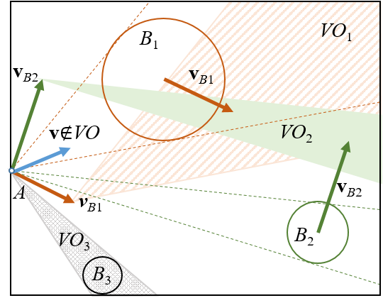Figure 1. Velocity obstacles for a point robot A with two moving (B_1,B_2) and a static obstacle (B_3). v_B1,v_B2 are the velocities of the obstacles. VO_i denotes the velocity obstacle corresponding to obstacle B_i. A collision-free example is depicted for robot velocity: v∉VO=⋃_(i=1)^3▒〖VO_i 〗.

Non-Linear Velocity Obstacles
The non-linear velocity obstacle (NLVO) defines the set of all linear robot velocities that would result a collision with obstacle B_i (t) moving along arbitrary known trajectory. At time instant t, one can define robot velocity vectors which move the robot to a position during time t-t_0 such that a collision occurs with B_i:
NLVO_i (t)=(c_i (t)+B_i)/(t-t_0 ) 3
where c_i (t) denotes the trajectory of the obstacle B_i. Considering all t>t_0, one gets
NLVO_i=⋃_(t>t_0)▒(c_i (t)+B_i)/(t-t_0 ) 4
The shape of the non-linear velocity obstacle NLVO_i is a warped cone with apex at A (see Figure 2). Similar to (2), the union of the individual NLVO_i defines the set of all robot velocity vectors which result a collision for some t>t_0.

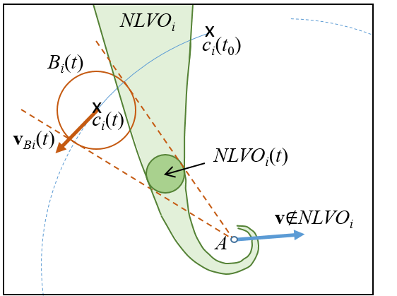Figure 2. NLVO for a point robot A with obstacle B_i moving along a circular path.

Generalized Velocity Obstacles
The concept of velocity obstacles was generalized to apply it for car-like robots [18]. The obstacle is defined in the control space of the robot:
GVO={u|∃t:‖A(t,u)-B(t)‖<r_A+r_B} 5
where u is the control input of the robot, A(t,u) is the position of A if control u was applied up to t. r_A and r_B denote the radii of the circular robot and obstacle.
The controls are sampled, and for each control u, the minimum distance between A and B is determined numerically, if control u was applied to the robot. If the minimum distance is smaller than the sum of the radii, u∈ GVO and it means that a collision will occur between B and A for the control u.
Idea for Extension
In this paper, the velocity obstacles are applied to similar robots as presented in Subsection 2.2. This solution will not be restricted to sampled control inputs, as suggested by [18]. The presented method represents the velocity obstacles for car-like robots as a subset of a two-dimensional plane similar to the methods of VO and NLVO. In this work, this plane is determined by the velocity of the robot and the curvature of its path.

3. Reeds-Shepp-Type Car-Like Mobile Robots

A car-like mobile robot (see Figure 3) can move in a two-dimensional workspace. The state of the robot is defined by its position and orientation. The position is given by the (x,y) coordinates of the midpoint of its rear axle. The orientation of the robot is denoted by θ, and it is defined by the angle of the positive x axis of the coordinate system and the longitudinal axis of the robot. Ackermann-steering is supposed (see [19]), and the movement of the robot is described by the motion of a bicycle putting on the longitudinal axis of the robot. The inputs of the robot are the longitudinal velocity v and the angle of the front turning wheel (δ). Notice, that v is a scalar.

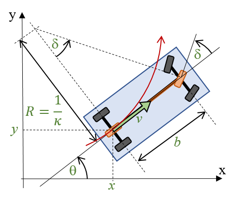Figure 3. Car-like mobile robot.

The kinematics of the robot reads:
[■(x ̇@y ̇@θ ̇ )]=[■(cos⁡θ@sin⁡θ@tan⁡δ/b)]v 6
where b is distance between the front and the rear wheels. The turning angle δ of the front wheel determines the radius R of the turning circle of the robot: R=b/tan⁡δ . The reciprocal of the turning radius is called curvature: κ=1/R=tan⁡δ/b.
The turning radius R cannot be arbitrary small, since the turning angle δ of the front wheels is also limited. Depending on the limit of δ and the geometrical b parameter of the robot, a minimal turning radius can be determined: R_min≤ |R|. Similarly, the curvature is also limited: |κ|≤κ_max.
The car-like mobile robot is a nonholonomic system since the direction of its velocity vector is constrained by the following equation:
x ̇ sin⁡〖θ-y ̇ cos⁡〖θ=0〗 〗 7
There are different types of car-like mobile robots: Dubins-robots can only move forward (i.e. v>0). It was proved that for given start and goal states the path with the minimal length consists of three segments: two or three circular segments with maximal curvature (i.e. with minimal turning radius) and, if needed, a straight-line between two circles if no obstacles are presented in the workspace [20]. The Reeds-Shepp-type mobile robots are able to travel both forward and backward. It was also shown that the path with minimal length between given start and goal states contains (like Dubins-robots) circular segments with maximal curvature, and it may contain straight-lines and cusp points where the driving direction changes [21].

4. Velocity Representation for Car-Like Mobile Robots

A Reeds-Shepp-type mobile robot can move forward or backward on a circular path segment with constant curvature (κ), i.e. with constant radius (R=1/κ), or on a straight-line. The curvature may have negative values, which shows that the robot turns in the negative direction (i.e. clockwise). The straight-line motion can also be described by a zero curvature. The time-distribution along the path depends on the longitudinal velocity v of the robot. The sign of v shows the direction of motion. These imply that the actual motion of the robot can be described by the pair (v,κ).
If (v,κ) is constant for a time period Δt, one can calculate the displacement in position and in orientation for Δt, if the motion starts at t_0=0 from [x_0,y_0,θ_0]=[0,0,0] by integrating (6):
[■(x(Δt)@y(Δt)@θ(Δt))]=[■(2/κ sin⁡〖κvΔt/2〗 cos⁡〖κvΔt/2〗@2/κ sin^2⁡〖κvΔt/2〗@κvΔt)] 8
This works in the reverse direction as well: if a point (x,y) is given in the workspace of the robot, one can determine the constant curvature κ and the constant forward longitudinal velocity v^f≥0 and backward velocity v^b<0, which can move the robot from t_0 = 0 and [x_0,y_0,θ_0]=[0,0,0] to this point during time Δt:
κ=2y/(x^2+y^2 ), 9
v^f=(x^2+y^2)/yΔt atan⁡〖y/x〗 10
v^b=(x^2+y^2)/yΔt (atan⁡〖y/x〗-sgn(atan⁡〖y/x〗 )π) 11
Notice, that (10) (and (11)) has several solutions for given x and y. If the robot does not go more than ones around in a circle, (10) (or (11)) will have a single solution for v^f (or for v^b) with -π <atan⁡〖y/x〗≤ π.
If the robot goes straight, its motion is described by: x=v Δt,y=0,κ=0,R=∞,v=x/Δt. In the sequel, the goal is to determine the (v,κ) (i.e. (v^f,κ) and (v^b,κ)) pairs which result a collision-free motion for the robot.

5. Velocity Obstacles for Car-Like Robots

Let the robot be at the [x_0,y_0,θ_0]=[0,0,0] initial state. First, such (v,κ) pairs are determined which result a collision with static obstacles. Then the collision with moving obstacles is also considered.

5.1 Collision with Static Obstacles

Suppose that a static obstacle is presented in the workspace of the robot. Let a circle represent the obstacle. Its position is given by the coordinates of its center: (x_o,y_o ) and its radius is r_o. For the sake of simplicity, the robot is also represented by a circle with radius r_r. (A non-circular robot or obstacle can be approximated by one or more circles.) To examine the collision for a point-like robot, the radius of the obstacle should be enlarged by the radius of the robot: r_o^’=r_o+r_r similar to the method proposed in [6].
First, such circular motions (i.e. curvatures κ_g) are considered, where the robot grazes (touches) the obstacle. Geometrically, the problem is the following: given a point (position of the robot), a straight-line going through this point (line of the robot’s orientation) and a circle (obstacle with enlarged radius r_o^’), such a circle has to be found, which is tangential to the circle of the obstacle and grazes the line of orientation at the given point (robot’s position).

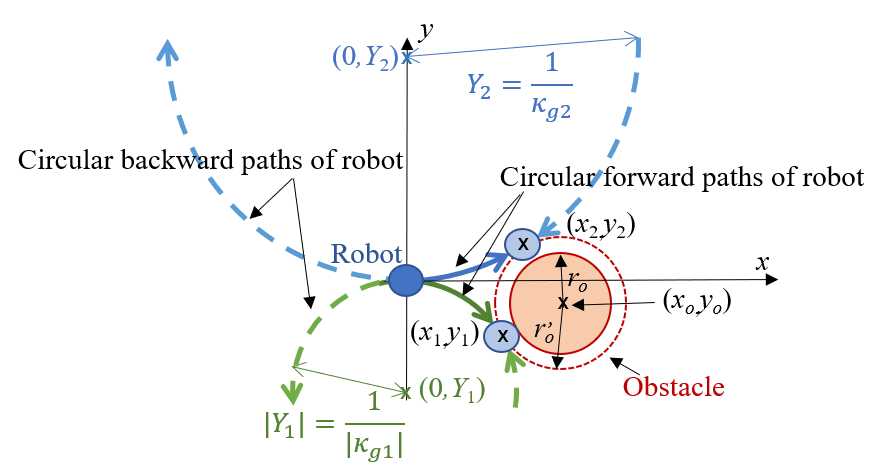Figure 4. Grazing a static obstacle.

There are two possibilities (see Figure 4). In both cases the center of the turning circle lies on the y-axis (i.e. the x coordinate of the center of the turning circle is 0). The y coordinate of the center of the turning circle defines the radius of the circle. The two possible values for the curvatures (or for reciprocals of y coordinates of the center) are:
κ_g1=1/Y_1 =2(y_o-r_o^’ )/(x_o^2+y_o^2-r_o^’2 ) 12
κ_g2=1/Y_2 =2(y_o+r_o^’ )/(x_o^2+y_o^2-r_o^’2 ) 13
All curvatures between κ_g1 and κ_g2 will result in a collision with the static obstacle. More precisely, moving on a circle with curvature κ_i≠0 will cause a collision if
min⁡〖(κ_g1,κ_g2 )<κ_i<max⁡〖(κ_g1,κ_g2)〗.〗 14
κ_i=0 can only cause a collision if
sgn (κ_g1 )≠sgn(κ_g2 )∧sgn(x_o )=sgn(v) 15
The coordinates of the grazing points ((x_1,y_1) resp. (x_2,y_2)) can be calculated as well:
x_1=(x_o (x_o^2+y_o^2-r_o^’2))/(x_o^2+(y_o-r_o^’ )^2 ), 16
y_1=((x_o^2+y_o^2-r_o^’2)(y_o-r_o^’))/(x_o^2+(y_o-r_o^’ )^2 ), 17
x_2=(x_o (x_o^2+y_o^2-r_o^’2))/(x_o^2+(y_o+r_o^’ )^2 ), 18
y_2=((x_o^2+y_o^2-r_o^’2)(y_o+r_o^’))/(x_o^2+(y_o+r_o^’ )^2 ). 19
Consider now the time instant t. The (v,κ) input pairs can be determined, which cause collision with the static obstacle B_i at t. The velocity obstacle for a car-like robot (VOCL) is the union of these points (see Figure 5):
VOCL_i (t)={ (v,κ)|A(t,v,κ)∩B_i≠∅} 20
where A(t,v,κ) represents the robot at time-moment t moving from t_0=0 and from the origin on a circular path with radius 1/κ with velocity v. κ and v can be calculated from (x,y) position using (9)-(11).

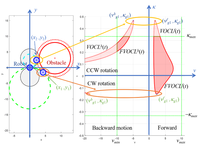Figure 5. a. Robot and obstacle at a grazing case. b. Velocity obstacle VOCL(t) and feasible VO FVOCL(t) for time instant

From the grazing points (x_1,y_1) and (x_2,y_2), one can determine the corresponding points in VOCL_i (t). The curvatures κ_g1 and κ_g2 are used and the forward velocities v_g1^f,v_g2^f and backward velocities v_g1^b,v_g2^b can also be calculated if (x_1,y_1) or (x_2,y_2) should be reached on a circular path during time t.
(v_g1,κ_g1) and (v_g2,κ_g2) lie on the boundary of VOCL_i (t). All other points on the boundary of VOCL_i (t) correspond to a motion (i.e. (v,κ) values) which moves the robot during time t to a boundary point of the obstacle, but before or after the time instant t a collision occurs.
VOCL_i (t) according to (20) may contain (v_j,κ_j) pairs, such that |κ_j |>κ_max or |v_j | > v_max. These κ_j or v_j values are not feasible. Feasible VO (FVOCL_i (t)⊆VOCL_i (t)) contains only feasible curvature and velocity values:
FVOCL_i (t)={(v,κ)|A(t,v,κ)∩B_i≠∅∧
|v|≤v_max∧ |κ|≤κ_max} 21

In Figure 5 VOCL_i (t) is delimited by dotted line and FVOCL_i (t) is bounded by solid line.

Taking time-moments in a time-interval t∈[t_0,t_h] one can get FVOCL_i for a static obstacle B_i:
FVOCL_i=⋃_(t∈[t_0,t_h])▒〖FVOCL_i (t)〗  22
If the robot moves according to (v,κ)∉ FVOCL_i, the robot will not collide with the static obstacle B_i in the given time interval [t_0,t_h].
Notice, that the selection of t_h influences the effectiveness and the computational demand of the method. If a small value was selected for t_h, a mobile robot may collide with a moving obstacle. On the other hand, a large time-horizon can result that VO includes almost the complete velocity space [13].

5.2Calculating VOCL for Moving Obstacles

For a moving obstacle B_i (t) the definition of VOCL_i (t) for a given time-moment t is similar to (20):
VOCL_i (t)={ (v,κ)|A(t,v,κ)∩B_i (t)≠∅} 23
FVOCL_i (t) and FVOCL_i can be determined as well, according to (21) and (22).
The main difference is the following: the grazing points in VOCL_i (t) ((v_g1,κ_g1) and (v_g2,κ_g2)) do not represent grazing cases any more if the obstacle is moving since the position of the grazing points depends on the motion of the obstacle.

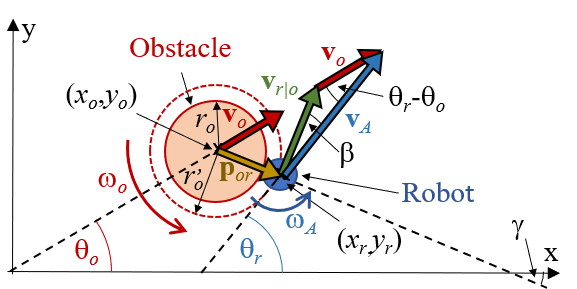Figure 6. Notations for moving obstacle at time instant t_A.

To analyze VOCL and the grazing points, the following notations are used (see Figure 6):
A time instant t_A is considered.
The position of the moving obstacle at t_A is denoted by (x_o (t_A),y_o (t_A)). The angle between the positive x-axis and the velocity vector v_o (t_A) of the obstacle is denoted by θ_o (t_A), the absolute value of the velocity is v_o (t_A). ω_o (t_A) denotes the turning rate of the obstacle. The vector ω_o (t_A) is parallel to the positive z-axis, if the direction of the rotation is positive, and to the negative z-axis in case of clockwise rotation.
An input pair (v_A,κ_A) is selected.
If a robot is moving with a velocity v_A on a circle with curvature κ_A for time t_A, its position (x_r (t_A),y_r (t_A)) and orientation θ_r (t_A) can be determined according to (8). The absolute value of the robot’s velocity v_A remains unchanged during the circular motion, but the vector of the velocity v_A (t_A) changes, since the orientation of the robot is also modified. The turning rate of the robot is ω_A=κ_A v_A. The direction of vector ω_A is parallel to the positive z-axis, if ω_A>0, and to the negative z-axis if ω_A<0. The vector ω_A is constant during the circular motion, since its direction and length (i.e. ω_A) are unchanged.
The relative velocity of the robot and the obstacle at time moment t_A is denoted by
v_(r|o) (t_A)=v_A (t_A)-v_o (t_A). 24
The angle between the velocity vector v_A (t_A) of the robot and the relative velocity v_(r|o) (t_A) is:
β(t_A )=atan⁡〖(v_o (t_A ) sin⁡〖(θ_r (t_A )-θ_o (t_A))〗)/(v_A-v_o (t_A ) cos⁡〖(θ_r (t_A )-θ_o (t_A))〗 )〗. 25
p_or is a vector connecting the center of the obstacle to the center of the robot.
The angle between the positive x-axis and p_or is:
γ(t_A )=atan⁡〖(y_r (t_A )-y_o (t_A))/(x_r (t_A )-x_o (t_A))〗 26
The following two propositions follow directly from the definition of VOCL_i (t).
Proposition 1:
√((x_r (t_A )-x_o (t_A ))^2+(y_r (t_A )-y_o (t_A))^2 )≤r_o^’⟺
(v_A,κ_A )∈VOCL_i (t_A) 27
If |κ_A |≤κ_max and |v_A |≤v_max, then (v_A,κ_A )∈ FVOCL_i (t_A) is also true. Similar to [14], the boundary points of the set VOCL(t) are denoted by δVOCL(t).
Proposition 2:
√((x_r (t_A )-x_o (t_A ))^2+(y_r (t_A )-y_o (t_A))^2 )=r_o^’⟺
(v_A,κ_A )∈δVOCL_i (t_A) 28
For the grazing points (v_g1,κ_g1) and (v_g2,κ_g2) in case of a static obstacle still holds true that (v_g1,κ_g1 )∈δVOCL_i (t_A) and (v_g2,κ_g2 )∈δVOCL_i (t_A) where δ denotes the region boundary. But these points are not grazing points any more, if the obstacle is moving.
Theorem 3: (v_A,κ_A) is a grazing point in VOCL_i (t_A) if
θ_r (t_A )+β(t_A )-γ(t_A )=(2a-1)π/2,a∈Z 29
Proof: θ_r (t_A)+β(t_A) denotes the angle between the relative velocity v_(r|o) (t_A) and the positive x-axis. γ(t_A) is the angle between the positive x-axis and p_or (the vector connecting the center of the robot and the obstacle). The condition for the grazing situation is that the relative velocity v_(r|o) (t_A) is perpendicular to p_or which is equivalent to the case where the relative velocity v_(r|o) (t_A) is tangent to the circle of the enlarged obstacle with radius r_o^’.
Similar to [14], it can be proven that if v_(r|o) (t_A) is perpendicular to p_or, the robot grazes the obstacle.
A point P is selected on the boundary of the robot. p_P is a vector which goes from the center of the robot to P. The velocity of the point P is:
v_P (t_A )= v_A (t_A )+ω_A×p_P 30
Similarly, a point Q can be selected on the boundary of the obstacle. p_Q is a vector which goes from the center of the obstacle to Q. The velocity of Q reads:
v_Q (t_A )=v_o (t_A )+ω_o (t_A )×p_Q. 31
If the point P of the robot grazes point Q on the obstacle, vector p_or has to be parallel to p_Q and -p_P. Moreover, grazing case can only occur, if the relative velocity of point P according to point Q is tangent to the circle of the obstacle, i.e. if it is perpendicular to p_or (and accordingly to p_Q and p_P as well). The relative velocity of P according to Q is:
v_(P|Q) (t_A)=v_P (t_A)-v_Q (t_A)=
=v_A (t_A )+ω_A×p_P-v_o (t_A )-ω_o (t_A )×p_Q 32
v_(P|Q) (t_A) is perpendicular to p_or, if:
v_(P|Q) (t_A )⋅p_or=0
(v_A+ω_A×p_P )⋅p_or-(v_o+ω_o×p_Q )⋅p_or= =0 33
Both (ω_A×p_P )⋅p_or and (ω_o (t_A )×p_Q )⋅p_or equal 0, hence one gets
(v_A (t_A )-v_o (t_A ))⋅p_or=0 34
which is equivalent to that v_(r|o) (t_A) is perpendicular to p_or.■
Notice, that the obstacles can move on arbitrary paths with arbitrary velocity profiles. The algorithm only supposes that for every time moment t_A∈[t_0,t_h] the positions and the velocity vectors of each obstacles are known.

5.3 Trajectories Avoiding Obstacles

If a goal position is given in the workspace of the robot, a motion should be planned which arrives to this point. During the motion, no collision should occur.
Fiorini and Shiller presented some heuristic search methods using Velocity Obstacles [6]. Applying these, one can easily select at each time moment a feasible velocity vector which moves the robot to the direction of the goal such that it avoids collisions with the obstacles. Using these heuristics alone does not guarantee to find an optimal solution. They designed an off-line global search method as well. A tree was generated for avoidance maneuvers using VO.
Shiller et al. presented avoidance maneuvers using NLVO [14]. These avoidance maneuvers can be used in a local or global motion planner as well.
The VOCL method can also be used in all above methods to plan the motion for car-like mobile robots to a given goal avoiding static and moving obstacles.

5.4 The Safest Solution

Another possibility for the selection of (v,κ) pair is to determine the safest motion. This method is called as the Safety Velocity Obstacles method (SVO).
The most important goal of the SVO method is to ensure the safest path for the robot during the motion.
This method checks, how far a possible (v,κ)∉FVOCL pair is from the nearest FVOCL_i (name this distance VO_dist). If the distance is bigger than a predefined threshold d_max, then the value of VO_dist is set to this maximum distance.
Hence, a normalized distance can be defined:
VO_norm=(VO_dist)/d_max 35
where VO_norm∈[0,1]. After that the value of the cost can be defined as
VO_cost=1-VO_norm 36
If the selected (v,κ) pair is far from the nearest FVOCL_i, then the value of VO_norm will be a big number (near to 1). So, such (v,κ) pair has to be chosen for the robot, where the value of VO_cost is minimal.
So, with the SVO method one can plan the safest motion in dynamic environment.

6. Simulation Results

An example for VOCL is presented here. A circular robot with radius r_o=0.9m is given. Its minimal turning radius is R_min=3m (i.e. κ_max=1/3 m^(-1) ) and its maximal velocity is v_max=7 m/s. Seven circular obstacles with different radii are presented in the workspace (see Figure 7). Four obstacles move (B_1,B_2,B_3,B_4) and there are three static obstacles (B_5,B_6,B_7). The velocity vectors and the paths of the dynamic obstacles are also depicted in Figure 7. The VOCL and FVOCL for t_h=10s is given in Figure 8. White areas represent (v,κ) pairs which correspond to collision-free motion for t_h.

Figure 7. An example with seven obstacles at t_0=0s. The velocity vectors of dynamic obstacles are depicted by solid lines, the paths of the obstacles are denoted by dotted lines (with t_h=10s).

A collision-free example is also presented here. κ=0.15m^(-1) (R=6.6 ̇m) and v=-5 m/s was selected. The corresponding (v,κ) point is depicted by a red star in Figure 8. The motion of the robot and the movement of the obstacles are depicted in Figure 9.

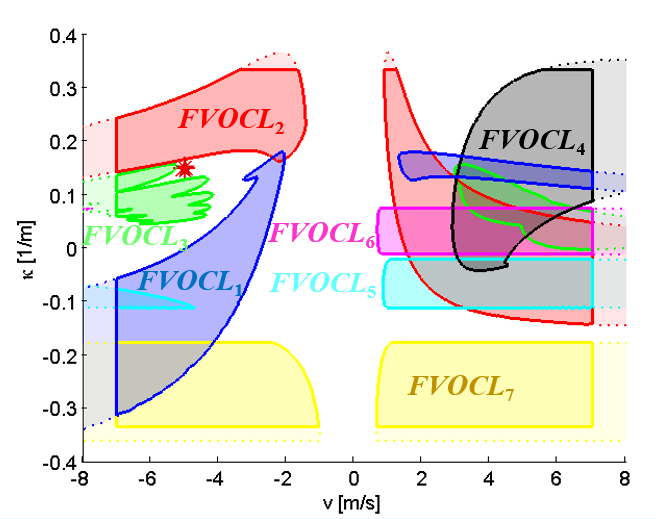Figure 8. Example for FVOCL=⋃▒〖FVOCL_i 〗 with seven obstacles.

7. Conclusion

Velocity obstacles (VO) and non-linear velocity obstacles (NLVO) methods can be used to plan a collision-free motion for a planar robot moving among static and moving obstacles. VO supposes that the obstacles move on straight-lines with constant velocities. If the path of the obstacle is not a straight-line, NLVO can be applied. These methods determine a velocity vector for the robot, which results in a collision-free motion in a time-interval. Applying this velocity, the robot will move on a straight-line according to the direction of the selected velocity vector. Both methods assume that the position and the motion of the obstacles are known.

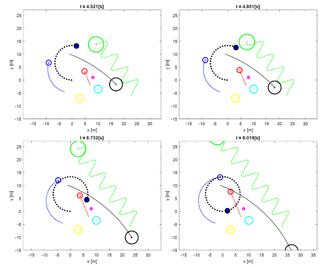Figure 9. Motion of robot and obstacles in the example (v=-5 m/s, κ=0.15m^(-1)). The robot is depicted by a blue disc, and its path is shown by the thick black dotted line.

The method, presented in this paper is similar to NLVO but in this case the robot is a car-like mobile robot. This robot cannot move to arbitrary direction. The direction of its velocity vector is determined by its orientation. The robot can move on a straight-line according to its orientation or on a circular path. Hence, the presented VOCL method determines only the magnitude of the velocity vector and, additionally, the curvature of the circular path to follow to avoid collisions. The next stage of this work is to implement the VOCL method for a car-like mobile robot, such that the collision-free motion is determined in real-time.
Our future goal is to take the non-circular shape of the robot (e.g. car-like rectangle) also into consideration during the construction of VOCL.
More feasible motion could be calculated if the path does not contain circular and straight-line segments only, but clothoid arcs as well as in [22]. In this case a continuous curvature path could be determined. The drawback is that the computational complexity would be larger.

1. Gincsainé Szádeczky-Kardoss, B. Kiss, “Velocity obstacles for Dubins-like mobile robots” in 25th Mediterranean Conference on Control and Automation (MED), Valletta, Malta, 2017. https://doi.org/10.1109/MED.2017.7984142
2. C. Latombe, Robot motion planning, Kluwer, Boston, 1991.
3. M. LaValle, Planning algorithms, Cambridge University Press, 2006.
4. Kant, S. W. Zucker, “Toward efficient trajectory planning: The path-velocity decomposition” Int. J. Robot. Res., 5(3), 72–89, 1986. https://doi.org/10.1177/027836498600500304
5. Szádeczky-Kardoss, B. Kiss, “Motion planning in dynamic environments with the rapidly exploring random tree method” Int. Rev. of Automatic Control, 1(1), 109–117, 2008.
6. Fiorini, Z. Shiller, “Motion planning in dynamic environments using velocity obstacles” Int. J. of Robot. Res., 17(7), 760–772, 1998. https://doi.org/10.1177/027836499801700706
7. Seder, I. Petrovic, “Dynamic window based approach to mobile robot motion control in the presence of moving obstacles” in International Conference on Robotics and Automation, Roma, Italy, 1986–1991, 2007. https://doi.org/10.1109/ROBOT.2007.363613
8. Khatib, “Real-Time obstacle avoidance for manipulators and mobile robots”. Int. J. Robot. Res., 5(1), 90–98, 1986. https://doi.org/10.1177/027836498600500106
9. Qixin, H. Yanwen, Z. Jingliang, “An evolutionary artificial potential field algorithm for dynamic path planning of mobile robot” in IEEE/RSJ International Conference on Intelligent Robots and Systems, Beijing, China, 3331–3336, 2006. https://doi.org/10.1109/IROS.2006.282508
10. Shi, J. N. Hua, “Mobile robot dynamic path planning based on artificial potential field approach” Adv. Mat. Res., 490–495, 994–998, 2012. https://doi.org/10.4028/www.scientific.net/AMR.490-495.994
11. Fox, W. Burgard, S. Thrun, “The dynamic window approach to collision avoidance” IEEE Robot. Autom. Mag., 4(1), 23–33, 1997. https://doi.org/10.1109/100.580977
12. Fraichard, H. Asama, “Inevitable collision states – a step towards safer robots?” Adv. Robotics, 18(10), 1001–1024, 2004. https://doi.org/10.1163/1568553042674662
13. Martinez-Gomez, T. Fraichard, “Collision avoidance in dynamic environments: an ICS-based solution and its comparative evaluation” in IEEE International Conference on Robotics and Automation, Kobe, Japan, 100–105, 2009. https://doi.org/10.1109/ROBOT.2009.5152536
14. Shiller, F. Large, S. Sekhavat, C. Laugier, “Motion planning in dynamic environments: Obstacles moving along arbitrary trajectories”. in IEEE International Conference on Robotics and Automation, Seoul, South Korea, 3716–3721, 2001. https://doi.org/10.1109/ROBOT.2001.933196
15. Moon, W. Chung, “Trajectory time scaling of a mobile robot to avoid dynamic obstacles on the basis of the INLVO” Adv. Robotics, 27(15), 1189–1198, 2013. https://doi.org/10.1080/01691864.2013.819604
16. Kuwata, M. T. Wolf, D. Zarzhitsky, T. L. Huntsberger, “Safe maritime autonomous navigation with COLREGS, using velocity obstacles” IEEE J. Oceanic Eng., 39(1), 110–119, 2014. https://doi.org/10.1109/JOE.2013.2254214
17. Snape, J. v. d. Berg, S. J. Guy, D. Manocha, “The hybrid reciprocal velocity obstacle”. IEEE T. Robot., 27(4), 696–706, 2011. https://doi.org/10.1109/TRO.2011.2120810
18. Wilkie, J. v. d. Berg, D. Manocha, “Generalized velocity obstacles”. in IEEE/RSJ International Conference on Intelligent Robots and Systems, St. Louis, MO, USA, 5573–5578, 2009. https://doi.org/10.1109/IROS.2009.5354175
19. A. Wolfe, “Analytical design of an Ackermann steering linkage” J. Eng. Ind.- T. ASME, 11, 11–14, 1959.
20. E. Dubins, “On curves of minimal length with a constraint on average curvature, and with prescribed initial and terminal positions and tangents” Am. J. Math., 79(3), 497–517, 1957. https://doi.org/10.2307/2372560
21. A. Reeds, L. A. Shepp, “Optimal paths for a car that goes both forwards and backwards”. Pac. J. Math., 145(2), 367–393, 1990
22. Fraichard, A. Scheuer, R. Desvigne, “From Reeds and Shepp’s to continuous-curvature paths” in International Conference on Advanced Robotics, Tokyo, Japan, 585–590, 1999.

(Click to view)

(Click to view)