1. Introduction

Supervised learning is widely utilised in various applications. However, it is still quite limited method. The majority of applications need handcrafted engineering extraction of features by implementing different techniques. This means that the principal purpose is to represent the bio-signal by applying proper feature representation methods. Whenever significant features represent bio-signal, classification error should be anticipated to be lower than extracting features, which are not genuinely representing data. However, the general engineering handcrafted representation is still effortful and consumes a long time. Moreover, the standard feature extraction algorithm relies on researcher’s experience. Many proposed feature learning methods may be implemented to improve feature representation automatically and save both effort and time. The primary evaluation of the behaviour of implemented feature learning method is the classification error. Deep learning is considered the most common technique to implement feature learning. Rina Detcher was the first to introduce the fundamentals for both first and second order deep learning [1]. Deep learning is an essential division of machine learning that consists of a multilayer. The output of each layer is considered as features that will be introduced to the following cascaded layer [2]. Artificial neural networks use a hidden layer to implement each layer of multilayers that construct deep learning [3]. Fig.1 shows a simple architecture of deep learning steps. The learning technique is done in a hierarchal method starting from the lower layers to the upper ones [4]. Deep learning can be used for both supervised and unsupervised learning where it learns features from data and eliminates any redundancy that might be existing in the representation. Unsupervised learning recruitment brings more defy than supervised one. Unsupervised learning for deep learning was implemented by Neural history compressors [5]and deep belief networks[6].

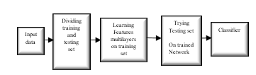­­Fig.1. Traditional Deep Learning Steps

This paper is organised by presenting a brief study on previous work that has been done on classification finger movement and deep learning in different fields, then a review study on autoencoder including the main equation for Auto-Encoder will be introduced. The surface electromyography will be assimilated by Wavelet Packet, Spectrogram and Wavelet. We will compare our results by implementing three different classifiers, which will be Support vector machine, Extreme learning machine with three activation functions and Softmax layer.

The Analysis of Variance (ANOVA) will be calculated for different classifiers in Auto-Encoder deep learning method. Also, the confidence interval for Auto-Encoder will be implemented as well. At last, each of training and testing accuracy will be promoted by concatenating classifier fusion layer.

2. Previous Work

In this research, we will suggest a deep learning system that will be capable of providing essential features from the input signal without recourse to traditional feature extraction and reduction algorithms. The suggested system will be talented in assert the ten hand finger motions.  The classification of different Finger motions was discussed earlier in many published scientific types of research. The early pattern recognition for finger movements was proposed in [7] where the researchers suggested using neural networks in analysing and classifying the introduced EMG pattern. They classified both finger movement and joint angle associated with moving finger. Later, in [8] the authors investigated and optimised configuration between electrode size and its arrangement to achieve high classification accuracy. Then, in [9] the researchers gave more attention to selecting the extremely discriminative features by employing Fuzzy Neighbourhood Preserving Analysis (FNPA) where the main purpose of this technique is to reduce the distance between the samples that belong to the same class and maximise it between samples of different classes. In the same year, other researchers explored the traditional machine learning well-known algorithm. Where, they used time domain features and implemented support vector machine, linear discriminate analysis and k-nearest neighbours as different classifiers then, they took advantage of   Genetic Algorithm to search for redundancy in the used dataset and selected features as well [10]. In the same context, authors proposed an accurate finger movement classification system by extracting time domain-auto regression features, reducing features by using orthogonal fuzzy neighbourhood discriminant analysis technique and implementing linear discriminant analysis as classifier [11]. After that, other researchers suggested an accurate pattern recognition system for finger movement by extracting 16-time domain features to process the Electromyography signal and implementing two layers feed forward neural networks as classifiers [12]. In contrast, effort and time that are being wasted, as mentioned before, in feature extraction and reduction were the motivation behind introducing the concept of deep learning. Therefore, many researchers published valuable achievements in deep learning for the biomedical signal. An extensive review study was presented on different types of research that recalled deep learning in health field [13]. The common factor in each study was the recruitment of neural network to learn features from input bio-signal. In the same context, researchers proposed a model by using convolutional neural networks to convert the information which was given by wearable sensor into highly related discriminative features [14]. Another research presented a deep learning record system that predicted the future medical risk automatically after extracting essential features by implementing convolutional neural networks [15]. Also, researchers implemented a system that used to extract shallow features from wearable sensor devices then the features were introduced to convolutional neural networks and finally to the classifier layer [16]. Based on the above, we can conclude that deep learning is an initial step towards implementing self-learning system by using neural networks. In our proposed system, we will implement neural networks in the form of two stages autoencoder, which read represented bio-signal by either spectrogram, wavelet or wavelet packet. We will use different classifiers to evaluate our system behaviour. Finally, we will add classifier fusion layer, which will follow best local classifier methodology. Adding classifier fusion was a promising contribution to the accuracies. Moreover, both confidence interval and Analysis of Variance will be estimated for different classifiers.

3. Sparse Auto-Encoder

An Autoencoder is an extensively used technique to reduce dimensions [17]. Sparse autoencoder idea first started in [18]. Where it started to reduce the redundancy that may result from complex statistical dependencies. Building a neural network and train it by using sparse method penalty as mentioned in [19] and taking into account the number of hidden nodes in the developed neural network, is considered a straightforward factor but as crucial as choosing the learning algorithm [20].

Auto-Encoder is a feed-forward neural network that is used in unsupervised learning [21]. The implemented neural network is being trained to learn features and produce it as its output rather than generating classes in case of recalling the classification ability of the hired neural network [22]. The encoder input is the represented data while its output is the features learnt by autoencoder. The learnt features learnt from the autoencoder will be introduced to classifier to be used in the assort of the data into predefined classes[23]. Lately, autoencoder is commonly employed to extract highly expressing features from data.

Unlabelled data can be used to train an autoencoder where training is mainly interested in optimising the cost function. The cost function is mainly responsible for estimating the miscalculation that may occur in calculating the reconstructed copy of input at the output and the input data.

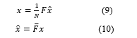
Assume that we have an input vector . The autoencoder maps this input to a new vector .

Where the superscript (1) represents the first layer of the autoencoder.  represents the transfer function,  represents the weight matrix, and  represents the bias vector. Then the decoder transfers the encoded representation  as a reconstruction of the input  following the next equation

Where the upper character (2) signifies the second layer of the autoencoder.  accounts for the transfer function,  represents the weight matrix, and  represents the bias vector.

The sparsity term can be introduced to autoencoder by adding an adapted cost function in the form of regularisation term. The regularisation function is estimated for each neuron  by averaging its activation function, which can be expressed as follows

Where  is the number of training samples,  is the  training sample of input,  is the   row of the weight matrix transpose of the first layer, and  is the  term of the bias vector for the neural network.  The neurone is considered to be firing if its output activation function is high and in the case of having a low activation value, this means that the neurone is only responding to a small number of input samples, which in turn encourages the autoencoder to learn. Accordingly, adding a limitation term to activation function output  limits every neurone to learn from limited features. This motivates the other neurones to respond to only another small number of features, which initiates every neurone to be responsible for responding to individual features for each input.

Introducing a sparsity regularise value is considered as a measure of how far or close is the targeted activation value  from the actual activation output function . Kullback-Leibler divergence is a very well know the equation that describes the difference between two different distributions. This equation is shown as follows:

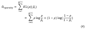The cost function is decreased to initiate the two distributions  and  to be as close as possible. The cost function can be represented by a mean square error equation as follows:

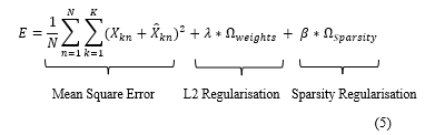Where L2 regularisation is a term to be added to the cost function to regulate and prevent the value of Sparsity Regularisation value of being small during the training due to the increase that may happen to the values of weights and decrease to the value of the mapped vector

 is the number of hidden layers,  is the number of input data samples, and  is the number of classes.

Autoencoder was hired in many research areas as a feature learning layer. Where its primary task, was to learn features from input data. A robust study was published to compare between many applications for autoencoder in deep learning field [24]. Autoencoder was implemented in [25] to learn incremental feature learning by introducing an extensive data set to denoising autoencoder. Denoising autoencoder provides an extremely robust performance against noisy data with a high classification accuracy [26, 27]. Another suggested autoencoder was a marginalised stacked one which showed a better performance, with high dimensional data, than the traditionally stacked autoencoder regarding accuracy and simulation time [28]. Denoising stacked autoencoder was hired to learn features from unlabeled data in a hierarchical behaviour [29] and was applied to filter spam by following greedy layer-wise to the implemented denoising stacked autoencoder [30].

In our proposed model, Auto-Encoder is a feed-forward neural network that is used in feature learning. The implemented neural network is being trained to learn features and produce it as its output rather than generating classes in case of recalling the classification ability of the hired neural network. Where, we implemented a stack autoencoder, which consists of two successive encoder stages. The input to the encoder is the data while the output is the features or representations. The classifier uses features produced from encoder as an input while; its output is the classes equivalent to input data [23]. Fig.2 demonstrates the steps that the surface electromyography signal moves through by using a sparse autoencoder.

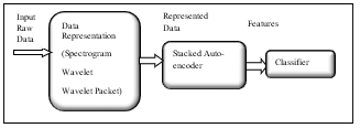Fig.2. Procedures of Sparse Auto-Encoder signal representation
In the same context of feature learning, autoencoder will generate useful features at the output, rather than producing classes, by decreasing the dimension of the input data into a lower dimension. However, the new lower dimension data will be dealt with our features that contain essential and discriminative information on the data, which will help in better classification results. Sparse autoencoder enhances us to leverage the availability of data.

4. Bio Signal Representation

We suggested three signal representations be applied on raw biological data to ensure fidelity and precision of our bio signal. Moreover, introducing raw data directly to first auto-encoder stage resulted in accuracy less than 50%. The first data representation was the spectrogram for bio raw signal. The spectrogram is interpreted to be the illustration of the spectrum of frequencies of our surface electromyography signal in a visible method. Numerically, Spectrogram can be estimated by calculating the square of the magnitude of Short-Time Fourier Transform (STFT). It can be called short-term Fourier transforms rather than spectrogram. In short time Fourier transforms, the long-time signal is divided into equal length segments and shorter in time.  Short time Fourier transforms is relevant to Fourier transform. Then, the frequency and phase for each segment to be estimated separately. Based on the above, we can deduce that spectrogram can be treated as  Fourier transform but for shorter segments rather than estimating it from the full long signal at once[31].

Assume that we have a discrete time signal  with a finite duration (limited signal) and a number of samples . The Discrete Fourier Transform (DFT) can be expressed as follows:

Knowing that the Fourier transform is estimated at frequency

The original signal  can be restored back from by applying the inverse Discrete Fourier Transform as follows:

The above-mentioned two equations can be rephrased as follows:

Where  is Fourier matrix of   dimensions and  is its complex conjugate

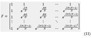Where the entries of  is expressed in terms frequencies coefficients

We need to calculate the spectrogram of the signal. Assume that we have a signal  of length , which is divided into successive equal segments . Where . The matrix of successive equal segments can be expressed as  where . The first column of   matrix equals  and its second column equals . The spectrogram for a signal  with window size  can be annotated . The columns which are composing matrix  is the discrete Fourier transform

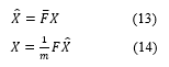The rows of the matrix  are representing the signal  in the time domain while its columns are representing the signal  in the frequency domain. So simply spectrogram is a time-frequency representation of the signal .

The spectrogram was used in many applications especially for speech signal analysis wherein [32] the authors represented the speech signal by different representations like Fourier and spectrogram to conclude that the resolution is mainly dependent on used representations. In [33] the researchers estimated the time corrected version of rapid frequency spectrogram of the speech signal which showed a better ability to follow the alterations in the bio-signal than other published techniques.

 The second signal representation used was wavelet of the signal. Wavelet is estimated by shifting and scaling small segmentations of the bio-signal. Fourier transform is an illustration of the signal in a sinusoidal wave by using various frequencies while wavelet is the illustration of the abrupt changes that happen to the signal. Fourier transform is considered a good representation of the signal in case of having a smooth signal. While wavelet is believed to be a better representation, than Fourier, for the sudden changing signal. Wavelet gives the opportunity to represent rapid variations of the signal and help the system extract more discriminative features.  We implemented Haar wavelet for our proposed model.

So in brief, a wavelet is an analysis for time series signal that has non-stationary power at many frequencies [34]. Assume that we have a time series signal  with equal time spacing  and  where the wavelet function is  that depends on time . The wavelet signal has zero mean and is represented in both time and frequency domain [35]. Morlet wavelet can be estimated by modulating our time domain signal by Gaussian as follows:

Where  is the frequency of the unmodulated signal. The continuous wavelet of a discrete signal  is the convolutional of  with scaled and shifted version of

Where * is the complex conjugate and  is the scale.

The wavelet transform was applied in several studies and different fields as in [36] where wavelet implemented in Geophysics field, in [37, 38] for climate, in [39] for weather, in [40]  and many other applications. The above equation can be simplified by reducing the number of . The convolutional theorem permits to estimate  convolutional in Fourier domain by implementing Discrete Fourier Transform (DFT). The Discrete Fourier Transform for .

Where  which is representing the frequencies. For a continuous signal ) is defined as . Based on the convolutional theorem, the inverse Fourier transform is equal to wavelet transform as follows:

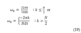
Where the angular frequency  can be expressed as follows:

An improved copy of wavelet algorithm was recalled in [41] where the authors presented two techniques. The first one used expansion factors for filtering while the other one is factoring wavelet transform. The researchers in [42] introduced the Morlet wavelet to vibration signal of a machine. The vibration signal of the low signal to noise ratio was represented by wavelet to grant fidelity to the signal and allow extraction better powerful features.  This model was implemented in [43] where researchers used wavelet transform to predict early malfunction symptoms that may happen in the gearbox.

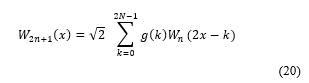
As a refinement act, we scaled the wavelet signal by five in wavelet, which in turn promoted the results as shown in Table I. As a comparative study, we utilised wavelet packet for the signal representation. The signal can be represented in both time and frequency domain simultaneously. This representation gains a fidelity to the signal due to its robust representation. Wavelet packet is one of the very widely used signal representation that produces the signal in both time and frequency domain [44]. The wavelet packet shows a very well acted for both nonstationary and transient signals [45-47]. Wavelet packet is estimated by a linear combination of wavelets. The coefficients of linear combination are calculated by recursive algorithm [48]. The wavelet packet estimation can be done as follows:

Assume that we have two wavelets type signal ,  and two filters of length . Let us assume that the following sequence of functions is representing wavelet functions.

Where  is the scaling function,  is the wavelet function.

Where  is the scaling function,  is the Haar wavelet function.

Many researchers implemented wavelet packet as in [49]. The authors used wavelet packet to create an index called rate index to detect the damage that may happen to the structure of any beam. In the same context authors of [50] employed wavelet packet and neural networks to detect a fault in a combustion engine. The implemented wavelet packet was six levels for sym10 at sampling frequency 2 kHz.

5. Classifiers

In the implementation of Auto-Encoder as feature learning algorithm, we applied three different classifiers, where the first was Softmax layer, the second was Extreme learning machine, and the third was Support Vector Machine (SVM). We measured the accuracy of Linear support vector machine, Quad support vector machine, Cubic support vector machine, Fine Gauss support vector machine, Medium Gauss support vector machine and Coarse Gauss support vector machine and elected the support vector machine classifier that resulted in the highest accurate result. Furthermore, the appending of classifier fusion layer to nominate best local classifier which in return endorsed the accuracy values. Fig.3 shows the block diagram for our implemented autoencoder feature learning proposed model

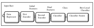Fig.3. Scheme of proposed Model

Moreover, ANOVA for autoencoder different classifiers was implemented. Where, we assembled average testing accuracies for four signal representation techniques (Wavelet, Wavelet Scale5, Wavelet Packet and Spectrogram) that resulted in P value 0.7487. So as wavelet results should not be counted, due to its low accuracy values, so, we suggested a second trial which was to group average testing accuracies for three signal representing techniques (Wavelet Scale5, Wavelet Packet and Spectrogram) that resulted in P value 0.3405. Both P values showed that there was no sensible variation between any of the implemented three classifiers as P value was higher than 0.05 in both cases. Fig.7 shows different P values for different classifiers.

In addition to the above, we estimated the confidence interval for each classifier. Our confidence interval was designed for confidence score 60%. Our assessed interval was bounded by higher and lower limit. In other words, we were confident or assured of any new accuracy by percentage 60% as long as it is located in the previously estimated interval.

6. Implementation

In this part, the data acquisition methods we followed will be expressed more extensively, and simulation outcomes will be exhibited and discussed.

6.1.  Data Acquisition

The surface Electromyography signal was read by using FlexComp Infiniti™ device. Two sensors were placed on the forearm of the participant of type T9503M. The placement of two electrodes on participant’s forearm is as shown in fig.4

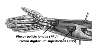Fig.4. Placement of the electrodes

The Electromyography signal was collected from nine participants. Each participant performed one finger movement for five seconds then had a rest for another five seconds. Every finger motion was reiterated six times. The same sequence was repeated for the second finger activity. Amplification of the signal by 1000 was applied and a sampling rate of 2000 samples for each second was implemented.

The collected Electromyography signal was used to categorise between predefined ten finger motions, as shown in Fig.5 via using our suggested model. Three folded cross validation was applied on our collected Electromyography signal. Accordingly, 2/3 of the collected data was assigned to training set while remaining 1/3 to be used by testing set.

Our surface electromyography signal was filtered to ensure fidelity and removal of any noise that may be inserted into the collected bio-signal. The average training or testing accuracy was estimated by simulating our proposed model for every subject apart then summed the accuracies for all subjects and divided the result by the total number of subjects.

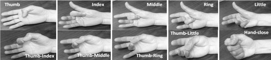Fig.5. Targeted Ten different finger motions

6.2.  Results

We implemented 400 nodes for the first layer of autoencoder and 300 nodes for the second one. As for the transfer function of the encoder, it was the pure linear type.

Table I shows autoencoder feature learning testing and training accuracy where the bio-signal was presented by spectrogram, wavelet, Wavelet scale 5 and wavelet packet. Three different classifiers were executed. The first was a SoftMax layer. While the second classifier was an extreme learning machine, we examined the performance of various activation functions for extreme learning machine classifier like sigmoid, the rectified linear unit and radial basis function. As that, the third classifier was support vector machine. We examined the performance of linear support vector machine, quadratic support vector machine, cubic support vector machine, fine gauss support vector machine, medium gauss support vector machine and coarse gauss support vector machine. Then, we selected the highest support vector machine that showed better classification ability to be our implemented support vector machine.

Table I. Auto Encoder Testing and Training Accuracy

Signal Representing	Average Training Accuracy	Average Testing Accuracy	Classification Algorithm	Simulation Time
Spectrogram	95%	73%	SoftMax Layer	830.93 Seconds
Spectrogram	95.5%	79.14%	ELM (Sigmoid)	379.10 Seconds
Spectrogram	95.5%	82.78%	ELM (ReLU)	379.54 Seconds
Spectrogram	97.237%	83.56%	ELM (RBF)	353.756 Seconds
Spectrogram	89.48%	77.27%	Cubic SVM	1000.409 Seconds
Wavelet	91.42%	45.71%	SoftMax Layer	210.04 Seconds
Wavelet	79.95%	59.88%	ELM (Sigmoid)	265.23 Seconds
Wavelet	83.62%	64.73%	ELM (ReLU)	276.149 Seconds
Wavelet	81.98%	62.70%	ELM (RBF)	257.83 Seconds
Wavelet	70.29%	52.29%	Linear SVM	341.57 Seconds
Wavelet (Scale 5)	98.85%	82.13%	SoftMax Layer	668.355 Seconds
Wavelet (Scale 5)	95.65%	85.416%	ELM (Sigmoid)	402.647 Seconds
Wavelet (Scale 5)	96.98%	86.827%	ELM (ReLU)	276.697 Seconds
Wavelet (Scale 5)	95.59%	85.58%	ELM (RBF)	444.067 Seconds
Wavelet (Scale 5)	96.55%	83.85%	Cubic SVM	495.124 Seconds
Wavelet Packet	98.69%	84.176%	SoftMax Layer	429.52 Seconds
Wavelet Packet	93.3%	86.79%	ELM (Sigmoid)	419.27 Seconds
Wavelet Packet	96.42%	89.41%	ELM (ReLU)	419.27 Seconds
Wavelet Packet	95.59%	87.78%	ELM (RBF)	540.22 Seconds
Wavelet Packet	98.16%	89.707%	Quad SVM	579.713 Seconds

From The above-shown results, we can explore that the classification ability for Extreme learning machine was outstanding in our application for all signal representation except for wavelet packet. Both quadratic support vector machine and extreme learning machine, with the rectified linear unit as an activation function, showed a very close performance for wavelet packet signal representation. Extreme learning machine was improved when we replaced sigmoid activation function by Radial basis function and the rectified linear unit. The rectified linear unit activation function for extreme learning machine presented a superior behaviour than radial basis function and sigmoid activation functions for wavelet, Wavelet scale 5 and wavelet packet. However, the rectified linear unit offered better performance than sigmoid and lower accuracy than radial basis function for spectrogram.

Cubic and Quad support vector machine started to result in a good testing accuracy for Wavelet scale 5 and wavelet packet only. Simulation time for support vector machine is relatively longer than other compared classification algorithms. SoftMax layer resulted in a very poor classification for wavelet signal representation, as the testing accuracy was less than 50%. Softmax started to prove its classification ability for Wavelet scale 5 and wavelet packet. Fig.6 shows different P values for different classifiers and Fig.7 shows confidence intervals for each classifier where it was calculated twice. The grey bars were calculated for different classifiers with three signal representation methods (Wavelet Scale5, Wavelet Packet and Spectrogram). While, yellow bars calculated for different classifiers with four signal representation methods (Wavelet, Wavelet Scale5, Wavelet Packet and Spectrogram). The narrowest interval was 2.53% for the extreme learning machine. While the widest one was 6.10% for support vector machine and softmax layer interval reached 5.77%.

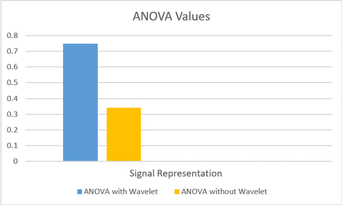Fig.6. ANOVA values for different Classifiers

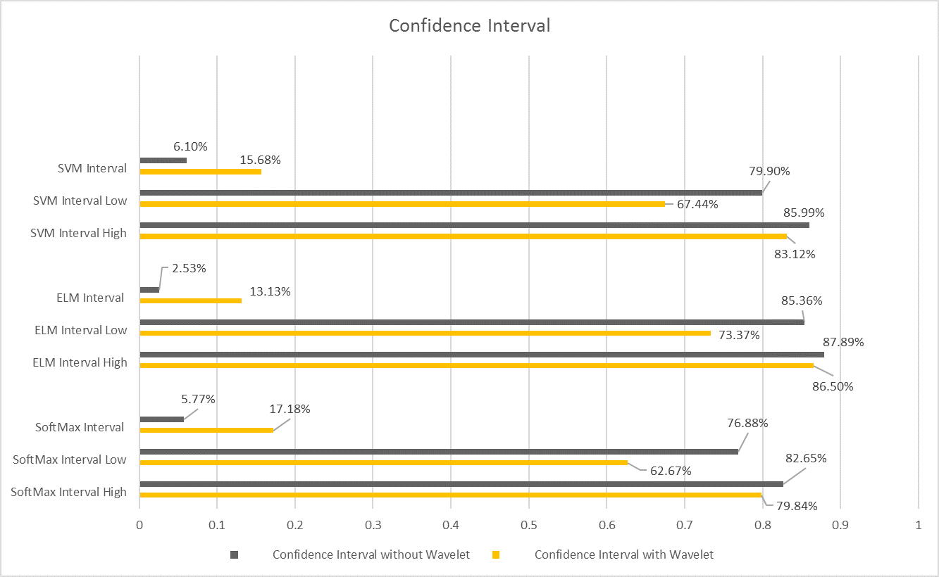Fig.7. Confidence Intervals for used classifiers

We concatenated a layer of classifier fusion after classification layer. The function of this added layer is to nominate the best-implemented classifier based on the outcomes of accuracies values. This added classifier fusion layer in return enriched our accuracies as displayed in Table II. On the other side, adding classifier fusion layer relatively increased the simulation time than without fusion layer.

Table II: Auto Encoder Classifier Fusion Testing and Training Accuracy

Signal Representing	Average Training Accuracy	Average Testing Accuracy	Classification Algorithm	Simulation Time
Spectrogram	99.53%	91.05%	Classifier Fusion	2118.846 Seconds
Wavelet	96.99%	86.80%	Classifier Fusion	745.67 Seconds
Wavelet (Scale 5)	99.24%	89.02%	Classifier Fusion	1378.41 Seconds
Wavelet Packet	98.70%	92.25%	Classifier Fusion	1656.724 Seconds

7. Conclusion

Sparse autoencoder is just one hidden layer algorithm. Therefore, to establish the concept of deep learning, and take advantage of stacking more than a layer, as the testing set accuracy was less than 50% for one stage only of the autoencoder, we implemented stacked autoencoder that led to verifying deep learning concept and enriching the results accuracy. In addition, applying some signal representation like calculating spectrogram, wavelet and wavelet packet, instead of using raw signal, and introducing the output of these signal representation to the first stage of autoencoder enhanced the performance of the system. Extreme learning machine showed a satisfactory performance on the level of testing accuracy and simulation time. Softmax layer classification resulted in the most mediocre testing accuracy although it consumed longer simulation time than extreme learning machine. Support vector machine produced an excellent testing accuracy but consumed long simulation time. Applying signal representation like Spectrogram, wavelet or wavelet packet improved both training and testing accuracy a lot as both accuracies were much less than 50% when we fed first stage autoencoder by raw data. Multiplying wavelet scale by 5 enhanced the results a lot. As a conclusion, applying any signal representation either in the time domain, frequency domain, or both had a good impact on our training and testing accuracies. We introduced the rectified linear unit as an activation function for extreme learning machine besides already existing functions such as radial basis function and sigmoid. The rectified linear unit was superior in its testing accuracy than both radial basis function and sigmoid one for wavelet, Wavelet scale 5 and wavelet packet signal representation. Moreover, it resulted in a lower testing accuracy than radial basis function but better than sigmoid for spectrogram signal representation.

Moreover, calculating ANOVA gave us an indication on how relative or far was different classifiers. The computation of confidence interval with confidence score 60% gave us the upper and lower accepted accuracies. Adding a classifier fusion layer was very helpful in improving the percentages of our accuracy in either the training set or the testing set. However, it consumed a long simulation time in comparison to without fusion layer. In Conclusion, deep learning was an initiative step towards saving effort and time wasted in extracting and reducing features as it learnt, by itself, the best features suitable for the application under examination. In addition, since feature extraction and reduction methods varied according to the application so, feature extraction and reduction algorithms were not fixed and needed more experience. In other words, deep learning system should be adaptable to any set of data if the data was accurate and well represented. This brought a new challenge on the scene in regarding representing the data. The data should be represented in a high precision way to expect a good result from implementing deep learning technique.

1. R. Dechter, “Learning While Searching in Constraint-Satisfaction-Problems,” presented at the Proceedings of the 5th National Conference on Artificial Intelligence, Philadelphia, 1986.
2. L. Y. Deng, D, “Deep Learning: Methods and Applications,” Foundations and Trends in Signal Processing, vol. 7, pp. 3-4, 2014.
3. Y. Bengio, “Learning Deep Architectures for AI,” Foundations and Trends in Machine Learning, vol. 2, no. 1, pp. 1-127, 2009.
4. Y. C. Bengio, A.; Vincent, P., “Representation Learning: A Review and New Perspectives,” IEEE Transactions on Pattern Analysis and Machine Intelligence, vol. 35, no. 8, pp. 1798–1828, 2013.
5. J. Schmidhuber., “Learning complex, extended sequences using the principle of history compression,” Neural Computation, vol. 4, pp. 234–242, 1992.
6. G. E. Hinton, “Deep belief networks,” Scholarpedia, vol. 4, no. 5, p. 5947, 2009.
7. A. H. Noriyoshi Uchida, Noboru Sonehara, and Katsunori Shimohara, “EMG pattern recognition by neural networks for multi fingers control,” presented at the Engineering in Medicine and Biology Society, 1992 14th Annual International Conference of the IEEE, 1992.
8. E. M. a. L. M. Alex Andrews, “Optimal Electrode Configurations for Finger Movement Classification using EMG,” presented at the 31st Annual International Conference of the IEEE EMBS, 2009.
9. S. K. Rami N. Khushaba, Dikai Liu, Gamini Dissanayake, “Electromyogram (EMG) Based Fingers Movement Recognition Using Neighborhood Preserving Analysis with QR-Decomposition,” presented at the 2011 Seventh International Conference on Intelligent Sensors, Sensor Networks and Information Processing (ISSNIP), 2011.
10. C. A. a. C. C. Gunter R. Kanitz, “Decoding of Individuated Finger Movements Using Surface EMG and Input Optimization Applying a Genetic Algorithm,” presented at the 33rd Annual International Conference of the IEEE EMBS, Boston, Massachusetts USA, 2011.
11. G. B. Ali H. Al-Timemy, Javier Escudero and Nicholas Outram, “Classification of Finger Movements for the Dexterous Hand Prosthesis Control With Surface Electromyography,” IEEE JOURNAL OF BIOMEDICAL AND HEALTH INFORMATICS, vol. 17, no. 03, pp. 608-618, 2013.
12. W. C. Mochammad Ariyanto, Khusnul A. Mustaqim, Mohamad Irfan, Jonny A. Pakpahan, Joga D. Setiawan and Andri R. Winoto, “Finger Movement Pattern Recognition Method Using Artificial Neural Network Based on Electromyography (EMG) Sensor,” presented at the 2015 International Conference on Automation, Cognitive Science, Optics, Micro Electro-Mechanical System, and Information Technology (ICACOMIT), Bandung, Indonesia, 2015.
13. C. W. Daniele Rav`i, Fani Deligianni, Melissa Berthelot, Javier Andreu-Perez, Benny Lo and Guang-Zhong Yang, “Deep Learning for Health Informatics,” IEEE JOURNAL OF BIOMEDICAL AND HEALTH INFORMATICS, vol. 21, no. 1, pp. 4-21, 2016.
14. T. K. Julius Hannink, Cristian F. Pasluosta, Karl-G ¨unter Gaßmann, Jochen Klucken, and Bjoern M. Eskofier, “Sensor-Based Gait Parameter Extraction With Deep Convolutional Neural Networks,” IEEE JOURNAL OF BIOMEDICAL AND HEALTH INFORMATICS, vol. 21, no. 1, pp. 85-93, 2016.
15. T. T. Phuoc Nguyen, Nilmini Wickramasinghe, and Svetha Venkatesh, “Deepr: A Convolutional Net for Medical Records,” IEEE JOURNAL OF BIOMEDICAL AND HEALTH INFORMATICS, vol. 21, no. 1, pp. 22-30, 2016.
16. C. W. Daniele Rav`i, Benny Lo, and Guang-Zhong Yang, “A Deep Learning Approach to on-Node Sensor Data Analytics for Mobile or Wearable Devices,” IEEE JOURNAL OF BIOMEDICAL AND HEALTH INFORMATICS, vol. 21, no. 1, pp. 56-64, 2016.
17. Y. Bengio, “Learning Deep Architectures for AI,” in “Foundations and Trends in Machine Learning,” Universit´e de Montr´eal, Canada2009.
18. D. J. F. BRUNO A OLSHAUSEN, “Sparse Coding with an Overcomplete Basis Set: Strategy Employed by V1?,” Pergamon, vol. 37, no. 23, pp. 3311-3325, 1997.
19. V. a. H. Nair, Geoffrey E, “In Advances in Neural Information Processing Systems,” presented at the Advances in Neural Information Processing Systems, 2009.
20. A. a. N. Coates, Andrew, “The importance of encoding versus training with sparse coding and vector quantization.,” in Proceedings of the 28th International Conference on Machine Learning (ICML-11), 2011, pp. 921–928.
21. Cheng-Yuan Liou, Jau-Chi Huang, Wen-Chie Yang, “Modeling word perception using the Elman network,” Neurocomputing, vol. 71, no. 16-18, pp. 3150-3157, 2008.
22. C.-Y. Liou, Cheng, C.-W., Liou, J.-W., and Liou, D.-R., “Autoencoder for Words,” Neurocomputing, vol. 139, pp. 84–96, 2014.
23. G. E. H. a. R. R. Salakhutdinov. (2006) Reducing the Dimensionality of Data with Neural Networks. SCIENCE.
24. F. V. Maryam M Najafabadi, Taghi M Khoshgoftaar, Naeem Seliya, Randall WaldEmail author and Edin Muharemagic, “Deep learning applications and challenges in big data analytics,” Journal of Big Data, vol. 2, no. 1, pp. 1-21, 2015.
25. S. K. a. L. H. Zhou G, “Online incremental feature learning with denoising autoencoders,” in International Conference on Artificial Intelligence and Statistics, 2012, pp. 1453–1461.
26. L. H. Vincent P, Bengio Y, and Manzagol Pierre Antoine, “Extracting and composing robust features with denoising autoencoders,” in 25th international conference on Machine learning, Helsinki, Finland, 2008.
27. H. L. Pascal Vincent, Isabelle Lajoie, Yoshua Bengio and Pierre-Antoine Manzagol “Stacked Denoising Autoencoders: Learning Useful Representations in a Deep Network with a Local Denoising Criterion,” The Journal of Machine Learning Research, vol. 11, no. 3, pp. 3371-3408 2010.
28. X. Z. Chen M, Weinberger KQ and Sha F, “Marginalized denoising autoencoders for domain adaptation,” in 29th International Conference in Machine Learning, Edingburgh, Scotland, 2012.
29. B. A. a. B. Y. Glorot X, “Domain adaptation for large-scale sentiment classification: A deep learning approach,” in 28th International Conference on Machine Learning 2011, pp. 513–520.
30. L. Y. a. F. Weisen, “Application of stacked denoising autoencoder in spamming filtering,” Journal of Computer Applications, vol. 35, no. 11, pp. 3256-3260, 2015.
31. I. D. Ervin Sejdic, Jin Jiang “Time-frequency feature representation using energy concentration: An overview of recent advances,” Digital Signal Processing, vol. 19, no. 1, pp. 153-183, 2009.
32. R. R. Mergu and S. K. Dixit, “Multi-resolution speech spectrogram,” International Journal of Computer Applications, vol. 15, no. 4, pp. 28-32, 2011.
33. S. A. Fulop and K. Fitz, “Algorithms for computing the time-corrected instantaneous frequency (reassigned) spectrogram, with applications,” The Journal of the Acoustical Society of America, vol. 119, no. 1, pp. 360-371, 2006.
    I. Daubechies, “The wavelet transform, time-frequency localization and signal analysis,” Information Theory, vol. 36, no. 5, pp. 961 – 1005, 1990.
34. M. Farye, “WAVELET TRANSFORMS AND THEIR APPLICATIONS TO TURBULENCE,” Fluid Mechanics, vol. 24, pp. 395–457, 1992.
35. H. W. a. K.-M. Lau, “Wavelets, Period Doubling, and Time–Frequency Localization with Application to Organization of Convection over the Tropical Western Pacific,” Journal of the Atmospheric Sciences, vol. 51, no. 17, pp. 2523–2541., 1994.
36. D. G. a. S. G. H. Philander, “Secular Changes of Annual and Interannual Variability in the Tropics during the Past Century,” Journal of Climate, vol. 8, pp. 864-876, 1995.
37. B. W. a. Y. Wang, “Temporal Structure of the Southern Oscillation as Revealed by Waveform and Wavelet Analysis,” Journal of Climate, vol. 9, pp. 1586-1598, 1996.
38. N. Gamage, and W. Blumen, “Comparative analysis of lowlevel cold fronts: Wavelet, Fourier, and empirical orthogonal function decompositions,” Monthly Weather Review, vol. 121, pp. 2867–2878, 1993.
39. P. F. Sallie Baliunas, Dmitry Sokoloff and Willie Soon, “Time scales and trends in the central England temperature data (1659–1990),” BrAVELET ANALYSIS OF CENTRAL ENGLAND TEMPERATURE vol. 24, pp. 1351-1354, 1997.
40. P. F. Sallie Baliunas, Dmitry Sokoloff and Willie Soon, “Time scales and trends in the central England temperature data (1659–1990),” BrAVELET ANALYSIS OF CENTRAL ENGLAND TEMPERATURE vol. 24, pp. 1351-1354, 1997.
41. A. Calderbank, I. Daubechies, W. Sweldens, and B.-L. Yeo, “Wavelet transforms that map integers to integers,” Applied and computational harmonic analysis, vol. 5, no. 3, pp. 332-369, 1998.
42. J. Lin and L. Qu, “Feature extraction based on Morlet wavelet and its application for mechanical fault diagnosis,” Journal of sound and vibration, vol. 234, no. 1, pp. 135-148, 2000.
43. J. Lin and M. Zuo, “Gearbox fault diagnosis using adaptive wavelet filter,” Mechanical systems and signal processing, vol. 17, no. 6, pp. 1259-1269, 2003.
44. M. V. Wickerhauser, “INRIA lectures on wavelet packet algorithms,” 1991.
45. R. P. a. G. Wilson, “Application of ‘matched’ wavelets to identification of metallic transients,” in Proceedings of the IEEE-SP International Symposium Time-Frequency and Time-Scale Analysis, Victoria, BC, Canada, Canada, 1992: IEEE.
46. E. S. a. M. Fabio, “The use of the discrete wavelet transform for acoustic emission signal processing,” in Proceedings of the IEEE–SP International Symposium, Victoria, British Columbia, Canada, 1992: IEEE.
47. T. P. T. Brotherton, R. Barton, A. Krieger, and L. Marple, “Applications of time frequency and time scale analysis to underwater acoustic transients,” in Proceedings of the IEEE–SP International Symposium, Victoria, British Columbia, Canada, 1992: IEEE.
48. M. Y. G. a. D. K. Khanduj, “Time Domain Signal Analysis Using Wavelet Packet Decomposition Approach ” Int. J. Communications, Network and System Sciences, vol. 3, pp. 321-329, 2010.
49. J.-G. Han, W.-X. Ren, and Z.-S. Sun, “Wavelet packet based damage identification of beam structures,” International Journal of Solids and Structures, vol. 42, no. 26, pp. 6610-6627, 2005.
50. J.-D. Wu and C.-H. Liu, “An expert system for fault diagnosis in internal combustion engines using wavelet packet transform and neural network,” Expert systems with applications, vol. 36, no. 3, pp. 4278-4286, 2009.

(Click to view)

(Click to view)