Introduction

Reliability assessment of safety-critical systems is becoming an almost insurmountable challenge. In the near future, the engineering of new applications for vehicles such as driving assistance functions or even autonomous driving systems will inevitably incur significantly increased engineering sophistication and longer test cycles. Thus, in the automotive domain, functional safety continues to be ensured on the basis of the international ISO 26262 standard. As both the levels of functionality such systems provide and their degree of interaction with their environment increases, an adequate increase in system safety assessment capabilities is required.

This paper is an extension of work originally presented at the 10th IEEE International Conference on Software Testing, Verification and Validation (ICST 2017) [1] and describes a methodology for efficiently assessing system safety. The focus of the paper is on regression testing of safety-critical systems consisting of black-box components. This scenario is common for automotive electronic systems, where testing time is expensive and should be reduced without an uncontrolled reduction in reliability.

The work reported here correspondingly seeks to increase testing efficiency by reducing the number of selected test cases in a regression test cycle. When a selection decision is made, the following two types of errors are possible:

• a test case is selected but would pass (type-Ierror, false-positive case) and
• a test case is not selected but would fail (type-IIerror, false-negative case).

Accordingly, we model a classifier Hˆ for solving the following optimization problem.

min pFP = P (Hˆ = H1|H0)  (1)

subject to pFN = P (Hˆ = H0|H1) ≤ pFN,MAX

A good standard of test efficiency calls for the avoidance of false-positives. This requires minimization of the probability of mistakenly assuming the rival hypothesis (H1 : test case fails) even though the null hypothesis (H0 : test case passes) is correct. Conversely, false-negatives mean that system failures remain undetected; the occurrence of this type of error must therefore be avoided with very stringent requirements. Thus, a predefined limit pFN,MAX for the probability of a false-negative is defined.

[1] proposed a concept for the selection of test cases based on a stochastic model. However, this paper proposes a holistic optimization framework for the safety assessment of safety-critical systems based on machine learning optimization techniques. We suggest an incrementally and actively learning linear classifier whose parameters are estimated on the basis of Bayesian inference rules. As a result, our novel approach for modeling a linear classifier outperforms other machine learning approaches in terms of sensitivity.

Furthermore, this paper deals with the following fundamentally important research question: The machine learning approach is trained with data (test evaluations) obtained during a concurrently running regression test. How much training data is enough? When does regression test selection actually start?

We extend the proposed selection method [1] by introducing suitable test case features that are used in the machine learning approach for increasing performance (see [2]). Therefore, each feature introduced increases the complexity of the optimization problem (cf. Eq. 1) as a new dimension for optimization is introduced. Thus [3] and [4] suggest that high dimensional optimization problems can be solved in reasonable timeframes by using evolutionary algorithms instead of a (grid)search-based approach as given in [1]. Accordingly, we propose an evolutionary optimization approach for increasing testing efficiency.

Further extensions, such as the introduction of a prioritization strategy for test cases in order to select higher-priority test cases, will also be presented within this paper. In our novel approach, a linear classifier is trained in an online session; the ordering of the training data on the basis of a prioritization strategy therefore has the potential to improve our classifiers’ performance.

We also provide an industrial case study to show the advantages of the suggested selection method. The study uses data from several regression test cycles of an ECU of a German car manufacturer, showing how test effort can be reduced significantly whereas the rates of both false-negatives and false-positives can be kept at very low values. In this example, we can quadruple test efficiency by keeping the falsenegative probability at 1%.

We first discuss related work in Sec. 2 and explain basic definitions in Sec. 3. Accordingly, we motivate our research topic in Sec. 4 by giving some background information on regression tests and referring to the challenges. In Sec. 5, we give a brief overview of known machine learning methods’ performance in solving safety-critical binary classification tasks. The concept of our novel machine learning approach is presented in Sec. 6. Sec. 7 discusses optimization strategies, and Sec. 8 focuses on the importance of the learning phase for the success of our approach. An industrial case study with real data is then given in Sec 9. Finally, Sec. 10 presents the paper’s conclusions.

2 Related Work

The automotive industry is currently engaged in a laborious quality assessment process around new engineered driver assistance and active and passive safety functions, while functional safety is ensured according to the international ISO 26262 standard [5]. Reliability assessment of systems is therefore, possible through both model-checking and testing.

Model-checking is used for verifying conditions on system properties. Thus [6] states that system requirements can also be validated by model-checking techniques. The idea is to check the degree to which system properties are met and to deduce logical conclusions on the basis of the satisfaction of system requirements. Model-checking has therefore gained wide acceptance in the field of hardware and protocol verification communities [7]. Motivated by the fact that numerical model-checking approaches cannot be directly applied to black-box components as a usable formal model is not available, we focus on modelchecking driven black-box testing [6] and statistical model-checking techniques [8]. However, there exist some approaches for interactively learning finite state systems of black-box components (see [9] and [10]), which are proposed as black box checking in [11]. Learning a model is an expensive task, as the interactively learned model has to be adapted due to inaccuracy reasons. Nevertheless, some assumptions about the system to be checked, such as the number of internal states, are necessary; furthermore, conformance testing for ensuring the accuracy of the learned model has to be iteratively performed [9].

Therefore, [8] outlines the advantages of statistical model-checking as being simple, efficient and uniformly applicable to white- and even to black-box systems. [6] motivates on-the-fly generation of test cases for checking system properties; here, a test case is generated for simulating a system for a finite number of executions. All these executions are used as individual attempts to discharge a statistical hypothesis test and finally for checking the satisfaction of a dedicated system property.

Model-checking driven testing, or even simply testing a system in order to validate its requirements, is an expensive task, especially where safety-critical systems are concerned. However, the focus is on regression testing, which means that the entire system under test has already been tested once but has to be tested again due to system modifications that have been carried out. The purpose of regression testing is to provide confidence that unchanged parts within the system are not affected by these modifications [12]. White-box selection techniques have been comprehensively researched [13, 14]. However, we are here considering black-box components, and hence selecting test cases that only check modified system blocks gets difficult.

Since the implementation of black-box systems and moreover, the information on performed system modifications is not available [12], reasonably conducting a regression test becomes impossible.

Accordingly, regression testing of safety-critical black-box systems ends up in simply executing all existing test cases; this is a retest-all approach [12].

This is also motivated by the fact that in the automotive industry, up to 80% of system failures [1] that are detected during a regression test have not occurred previously. The reason behind this fact is that often many unintended bugs are introduced during a bug-fixing process. So between two system releases many new unknown errors are often introduced.

For reducing the overall test effort, we apply a test case selection method [1] based on hypothesis tests. Those test cases that are assumed to fail on their executions are accordingly selected. However, type errors while performing hypothesis tests are possible, as, for instance, in statistical model-checking.

We extend the proposed selection method into a holistic machine learning-driven optimization framework that utilizes suitable test case features for increasing testing efficiency (see [2]). Machine learning methods are often trained in so-called batch modes. Nevertheless, many applications in the field of autonomous robotics or driving are trained on the basis of continuously arriving training data [15]. Thus, incremental learning facilitates learning from streaming data and hence is exposed to continuous model adaptation [15]. Especially handling non-stationary data assumes key importance in applications like voice and face recognition due to dynamically evolving patterns. Accordingly, many adaptive clustering models have been proposed, including incremental K-means and evolutionary spectral clustering techniques [16].

Furthermore, labeling input data is often awkward and expensive [17] and hence accurately training models can be difficult. Therefore, semi-supervised learning techniques are developed for learning from both labeled and unlabeled data [17]. Motivated by these techniques, we propose a similar approach for effectively learning from labeled data. Hence, we cluster binary labeled data in more than two clusters for improving a classifier’s learning capability due to the optimization of an objective function. Our optimization framework thus utilizes evolutionary optimization algorithms for handling the optimization complexity. Minimization of labeling cost on the basis of active learning strategies [18, 19] will also be dealt with in this paper.

3 Basic Definitions

We define the test suite T = {ti | 1 ≤ i ≤ M} consisting of a total of M test cases. TExec ∈ T and TExec  ∈ T are subsets of T that contain test cases that are executed and deselected in a current regression test respectively. Based on the test case executions (∀ti ∈ TExec), a system’s reliability is actually learned, and thus the machine learning algorithm is trained.

The focus in supervised learning is on understanding the relationship between feature and data (here test case evaluation) [4]. Therefore, a test case needs to code a feature vector so that the indication of the coded features for a system failure can be learned in a supervised fashion. Such an indication is not just a highly probable forecast of an expected system failure, it is rather a particular risk-associated recognition.

First of all, a feature can be any individual measurable property of a test case. The data type of a feature is mostly numeric, but strings are also possible. However, such features need to be informative, discriminative and independent of one another if they are to be relevant and non-redundant The definition of suitable features increases the classifier performance [20]. In our application, a feature can be varied, such as a

• subjective ranking of a test case based on expert knowledge. Such rankings can hint at the error susceptibility of verified parts of the system;
• verified function’s safety integrity level, known as the ASIL in automotive applications [5];
• name of a function whose reliability is assured;
• reference to any hardware component of a circuit board that is being tested in a hardware-inthe-loop (HiL) test environment;
• number of totally involved electronic control units during the testing of a networked functionality; Such a number can hint at the complexity of the networked functionality and hence at its error susceptibility.

We define the entire set of features Φ = {φf | 1 ≤ f ≤ F} of test cases that might be relevant for understanding the behavior of test cases. Thus, features may be e.g. φ1 = {0QM0,0 A0,0 B0,0 C0,0 D0} (ASIL) or φ2 = {f1, f2, f3} (function name). Hence, a test case can verify a function f3 that has an ASIL A.

The following passages discuss the selection of suitable features, which is an important strategy for improving a classifier’s performance.

• Sometimes less is more – If the defined set Φ is too large it can cause huge training effort, high dimensionality of the optimization problem and overfitting. Thus we define a selection mask h      i bs = 1 0 0···1 of length F for selecting relevant features Φs. If the f − th matrix entry of bs is greater than or equal to 1, then the corresponding feature φf ∈ Φ is selected and added to Φs, otherwise not.

• The set of main features Φm ⊆ Φs is coded as follows: If the f − th matrix entry of bs is equal to 2, then the corresponding feature φf ∈ Φs is at the same time a main feature φf ∈ Φm, otherwise not. The main features are used to establish the overall training data set: The training data is adapted to each test case, and thus it is Φm Tti = {tj | tj ∈ TExec ∧ ti ≡ tj}. Hence, we define Φ that two test cases ti and tj are equivalent ti ≡ tj if their features ∀φf ∈ Φ have identical values.

Additionally, a cross-product transformation of features ∀φf ∈ Φs \ Φm is performed. Thus we define Ψ = φf1 × φf2 × … × φfh × … × φfH with φfh ∈ Φs \ Φm,1 ≤ h ≤ H = |Φs \ Φm| consisting of features ψl that represent individual combinational settings for features φf ∈ Φs \ Φm. In simple terms, the cross-product of our sample features is φ1 × φ2 = {(0QM0,f1),(0QM0,f2),(0QM0,f3),(0A0,f1),…} Finally, a Boolean function check : T ×Ψ → B with check(ti,ψl) = (0,    if ti’s features are given by ψl) is defined.

In addition, the function state: T × R → S is defined; it returns the state of a dedicated test case in a concrete regression test. The state has to be either ’Pass’ or ’Fail’, except for cases where the test case has not been executed so that its state is undefined. Therefore, S = {’Pass’,’Fail’,’Undefined’} defines the set of possible states. Furthermore, the set R = {rk | 0 ≤ k ≤ K} includes r0 which is the current regression test and older regression tests starting from the last regression r1 to the first considered regression rK. Lastly, we define the tuple history(ti) = {state(ti,r1),…,state(ti,rK)} containing ti’s previous test results.

4 Motivation

In practice, finding suitable features is a difficult task. Since we focus here on black-box systems, systeminternal information is not available that might be useful for understanding the system behavior. As a reason, we can only define the above listed features, which might be too high-level for classifying system failures. To illustrate this fact, Fig. 1 a) shows a typical situation: The behavior of test cases in relation to arbitrarily defined features φ1 and φ2 is given. Passed and failed test cases are presented by green squares and red diamonds respectively, and white circles stand for test cases yet to be executed.

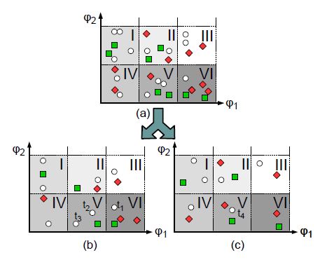Figure 1: An artificial regression test with test cases.

We can see that the green squares and the red diamonds are widely scattered. Thus, defining a hyperplane in order to set two acceptance regions for passing and failing test cases is no easy matter. In order to solve this complex task, we develop a novel approach that is basically motivated by the following thought experiment: All test cases that are represented in Fig. 1 a) are now either assigned to 1 b) or 1 c) according to a certain mapping. The individual mappings of test cases will be discussed later, in Sec. 6. In the next step, a cross-product transformation is performed in order to group test cases into sub-regions (we refer these later as sub-clusters). In our example, we create six sub-regions. Table 1 lists the empirical failure probabilities of each sub-region.

In order to keep our thought experiment very simple, we will neglect statistical computations for now and focus only on the main idea of our novel approach. The introduction of Bayesian networks and hence the derivation of weights for linear classifiers will be discussed later, in Sec. 6. We assume for now that the calculated failure probabilities of test cases in Fig. 1 b) and Fig. 1 c) are correlated. So our example remains very simple, we also require that the failure probabilities of the corresponding sub-regions are equal. This assumption reduces the complexity of the following classification task enormously. We will classify the following test cases t1, t2, t3 and t4 in accordance with whether a selection is necessary or not.

Table 1: Failure probability of each sub-region.

P (H1)             I              II             III            IV            V             VI

Fig. 1 a)           0             0.5          1             1             1/3         3/5

Fig. 1 b)          0             0.5          1             1             0             2/3

Fig. 1 c)           0             0.5          1             1             0.5          0.5

Only if t1 passes will the failure probability of subregion VI in Fig. 1 b) be equal to the failure probability of sub-region VI in Fig. 1 c). According to this fact, t1 is assumed to pass, and hence it is deselected. Furthermore, t2 will be selected as a fail of a test case inside sub-region V is expected. However, t2 passes, and, based on the same consideration, t3 is also selected and finally fails. Since now a failure probability of 1/3 is expected in sub-region V, t4 is assumed to pass, and therefore it does not need to be selected. Table 2 summarizes all decisions executed.

Table 2: Test case states and algorithm decisions.

Test Case        State      Decision Type of Decision

t1     Pass       Deselected           True-Negative

t2     Pass       Selected False-Positive

t3     Fail         Selected True-Positive

t4     Pass       Deselected           True-Negative

So our novel approach for solving binary classification tasks is based on calculated empirical probabilities and empirically evaluated correlations among those probabilities. The behavior of test cases can be precisely estimated on the basis of the calculated correlations. In practice, the failure probabilities of same sub-regions in Fig. 1 b) and Fig. 1 c) is often not exactly equal, but these failure probabilities are correlated. So the main task is to find good sub-regions for maximizing the empirically evaluated correlations and thus for precisely estimating the behavior of test cases. A more detailed explanation of our novel approach will follow in Sec. 6.

5 Performance of Known Machine Learning Methods

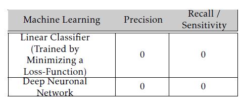
We have already indicated, by showing the example regression test in Sec. 4 (see Fig. 1), that according to the distribution of the input data, many machine learning methods cannot be reasonably applied for solving the constrained optimization problem (cf. Eq. 1). We will now demonstrate briefly that training linear classifiers in the classical sense by minimizing a loss function cannot perform well for solving safety-critical binary classification tasks. The situation is that only a small percentage of the data is actually labeled with one (’Fail’). Furthermore, failed and passed test cases are widely scattered in the feature space, which means detecting failing test cases becomes impossible. Additionally, the performance of deep neuronal networks is validated in the following.

The evaluation results (precision/recall) of these machine learning methods are given in Table 3. Each machine learning method is trained in the batch mode. The training data consists of all obtained test evaluations of a special regression test that will also be analyzed in our industrial case study in Sec. 9. For evaluating the machine learning methods, we used

the training data first for training and later for testing (training data = test data). Even so, the sensitivity of both machine learning methods is zero, and thus we propose a novel approach for determining a linear classifier’s parameters in Sec. 6.

Table 3: Performance of known machine learning methods in solving safety-critical binary classification tasks.

6 Concept

The concept of our novel approach is shown in Fig. 2. We start with specifying a feature set Φ, and taking its subset Φs and finally constitute a cross-product feature transformation to obtain the set Ψ . Based on Ψ and by applying the check-function on TExec, test cases can be grouped. If we look back to the example where we grouped test cases in Fig. 1 a), then we will see that there is a relationship between test cases’ features and their assignments to sub-regions.

Correspondingly, we introduce the definitions of clusters and sub-clusters of test cases. In the first step, test cases ∀tk ∈ Tti are assigned to clusters based on their history-tuples. A cluster is basically a partition of Tti and consists of test cases that have the same history-tuples. Accordingly, the number of distinct history-tuples N determines the total number of clusters. This is the step that has already been shown in Sec. 4, where test cases inside Fig. 1 a) were individually mapped into Figs. 1 b) and 1 c). In this way, already executed test cases depicted in Fig. 1 b) belong to one cluster and, analogously, those executed test cases that are depicted in Fig. 1 c) belong to another cluster.

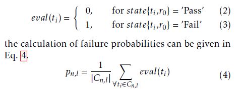
In the next step, each cluster Cn is subdivided into L sub-clusters. A test case tk ∈ Cn is an element of the l-th sub-cluster Cn,l if check(tk,ψl) is true. We originally introduced the terminology of sub-regions in Sec. 4. However, we focus in what follows on discrete valued features, which means that grouping test cases into sub-clusters is more appropriate. By introducing the function eval : TExec → {0,1} that is defined as follows

The given selection decisions in our example in Sec. 4 (cf. Fig. 1) were taken based on calculated failure probabilities. Additionally, the correlations between the failure probabilities were considered. Accordingly, we need a stochastic model for estimating the classifier’s sensitivity and specificity. We propose a univariate and also a multivariate stochastic model. The short-comings of the univariate stochastic model for solving the optimization problem (cf. Eq. 1) will be discussed later to motivate the introduction of a multivariate stochastic model. First of all, the next step introduces a multidimensional Gaussian distribution that constitutes a distribution for the failure probabilities of test cases. Based on this distribution, two distinct Bayesian Belief networks for both stochastic models will be introduced.

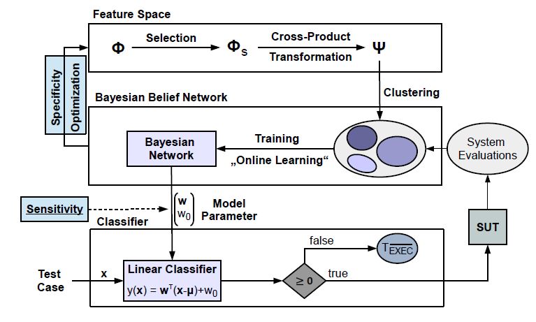Figure 2: Determining the weights of a linear classifier for maximizing its specificity under the constraint of a

In the following, we interpret pn,l,1 ≤ l ≤ L as realizations of a random variable Xn. Xn is Gaussian distributed based on the following assumption: specific sensitivity.

Since each test case evaluation is a binary experiment with two possible outcomes (’0’ or ’1’), it can be regarded as a realization of a binary random variable. As the sum of independent random variables results into a Gaussian random variable according to the central-limit theorem [21], considering test case evaluations as independent random experiments justifies Xn’s assumed distribution. However, test cases are executed on the same system and there may be some dependencies between test case evaluations that cannot be directly validated by such means as performing code inspections. As a result, we assume a mix of dependent and independent test case evaluations, and hence the Gaussian assumption is still valid. The moments of Xn are E[Xn] = µn = L1 PLl=1pn,l and E[(Xn −E[Xn])2] = σn2 = L−11 PLl=1(pn,l −E[Xn])2. As we introduced in total N Gaussian random variables, the moments of the multidimensional Gaussian distribution are µ = E[X] = [E[X1],E[X2],…,E[XN ]]T and Σ = E[(X − µ)(X − µ)T ].

Since the constraint of the optimization problem (cf. Eq. 1) has to be fulfilled, an accurate sensitivity estimation has to be iteratively performed.

6.1   Sensitivity Estimation

The formula for calculating the classifier’s falsenegative selection probability is given in Eq. 5.

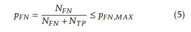
However, pˆFN = NˆFNNˆ+FNNT P has to be estimated, since the number of mistakenly deselected failing test cases NFN is unknown, and thus it is estimated by NˆFN . The number of already detected failing test cases is given by NT P . Before a decision can be taken on whether a test case ti can be deselected, the currently allowed risk of taking a wrong decision has to be estimated in advance. The estimation of NˆFN has to be adjusted by the term xP (Hˆ = H0|H1), where x is the failure probability of ti and P (Hˆ = H0|H1) is the estimated falsenegative probability if ti is deselected. Accordingly, the recursive formulation NˆFN,new = NˆFN,old + xP (Hˆ = H0|H1) is continuously updated whenever an arbitrary test case is deselected. As pˆFN ≤ pFN,MAX ⇔

NˆFN,newNˆFN,new+NT P ≤ pFN,MAX is required, the maximum allowed false-negative probability for deselecting the next test case ti is given in Eq. 6.

6.2 Univariate Stochastic Model

We model the Bayesian Network that consists of the random variables X, H and Hˆ , in Fig. 3. In the univariate stochastic model, the focus is on modeling of only one failure probability distribution. Thus the random variable X stands for the previously defined X1 and its realization x is given by p1,l where l is the index of that sub-cluster C1,l that fulfills ti ∈ C1,l.

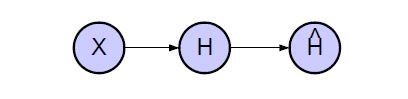Figure 3: Bayesian Network consisting of the random variables X, H and Hˆ .

H and Hˆ are binary random variables for modeling test case states and classifier decisions. As the state of a test case ti is a-priori unknown, it needs to be modeled by a corresponding random variable. According to the realization of X, a pass or a fail of the corresponding test case ti, whose failure probability distribution is modeled by X, is expected. Finally, Hˆ takes a decision for ti based on its failure probability x:

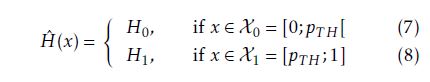
According to Hˆ ’s selection rule a very simple hyperplane y(x) = x − pT H is derived where in the case of y(x) ≥ 0 a selection decision is taken. A particularly important factor is the definition of the threshold probability pT H, as its setting determines the classifier’s sensitivity and specificity. The common ways of estimating false-negative and false-positive probabilities are given in equations 9 and 10, respectively.

 

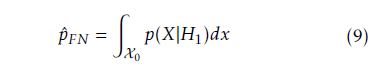
However, we could only estimate the probability density function (pdf) p(X) in contrast to the conditional probability density functions p(X|H0) and p(X|H1). The reason for this is that pdf estimations are based on mean calculations of test case evaluations. Hence passing and failing test cases are both considered in calculating average failure probabilities. Thus, p(X) is a distribution over failure probabilities of passing as well as failing test cases. Accordingly, p(X|H0) and p(X|H1) cannot be estimated and in conclusion, pˆFN and pˆFP cannot be estimated as in Eq. 9 and 10.

Z pˆFP =            p(X|H0)dx            (10)

Fig. 4 shows the important probability distribution functions that are used for estimating pˆFN and pˆFP .

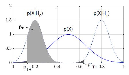Figure 4: Considered probability distribution functions in the univariate stochastic model.

The threshold probability pT H is calculated based on the estimation of pˆFN as the following relation in Eq. 11 holds.

pˆFN = P (X < p              (11)

As Eq. 11 cannot be directly estimated, the following relation in Eq. 12 is used for estimating pˆFN and finally for pT H.

pˆFN = P (X < pT H|H1) ≤ P (X < pT H) ≤ pFN,Limit (12)

pˆFN is estimated in Eq. 12 according to the assumption that the quantiles of p(X|H1) are larger than the quantiles of p(X). By solving Eq. 12 the threshold probability is computed as given in Eq. 13

√ pT H = erfinv(2pFN,Limit − 1)σ  2+µ        (13)

with µ = E[X] and σ = pV AR(X). As a result, the classifier’s sensitivity is larger than 1−pFN,Limit, since its false-negative selection probability is smaller than pFN,Limit. Finally, the decision regions of the linear classifier are defined (cf. Eq. 7 and 8) by determining pT H.

Furthermore, the minimization of the classifier’s specificity is required by the definition of the constraint optimization problem (cf. Eq. 1). Accordingly, the classifier’s false-positive selection probability is estimated as given in Eq. 14 and shown in Fig. 4.

pˆFP = P (X ≥ pT H|H0)                             (14)

However, p(X|H0) is not given and thus pˆFP cannot reasonably be estimated. Furthermore, pˆFP cannot be reasonably minimized as an optimization parameter is not defined; consequently, we need a so-called multivariate stochastic model for performing this. In the first instance, the idea of minimizing pˆFP and hence gaining testing efficiency by regarding several distribution functions is explained.

6.3   Preliminaries

Let us assume that two dependent Gaussian random variables X and X0 are given. The focus is again on estimating pˆFN and pˆFP . Fig. 5 shows the probability distribution functions p(X), p(X|H0) and p(X|H1) as in Fig. 4. Additionally, the a-posteriori failure probability distribution function p(X|X0) is shown.

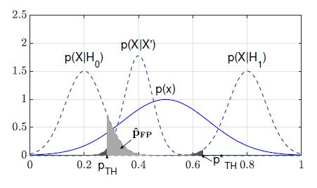Figure 5: Qualitatively minimizing pˆFP by introducing p(X|X0) and hence by using conditional informations.

The main idea is to use several observations of distinct dependent random variables to achieve a considerably more representative a-posteriori failure probability distribution function that is relatively narrow within a certain range. So p(X|X0) is considered as the more representative distribution for the failure probabilities and hence pˆFN and pT H are estimated by using this distribution function. Comparing Figs. 4 and 5, it can easily be seen that pˆFP is basically minimized, since the risk of a false-negative selection probability is computed based on p(X|X0), which allows a more representative risk estimation.

All in all, by regarding a set of dependent Gaussian random variables and by using the information about their observations, a more representative aposteriori failure probability distribution function is achieved, which allows a more precise risk estimation. Accordingly, the probability of false-positive selection can be minimized. As a result, a multivariate stochastic model is created to exploit the dependency information between random variables for finally achieving testing efficiency.

6.4   Multivariate Stochastic Model

By using the dependency between the random variables Xn,1 ≤ n ≤ N, a considerably more accurate estimation of pˆFN is achieved and hence pˆFP is minimized. Fig. 6 shows the modeled Bayesian network consisting of the random variables Xn,1 ≤ n ≤ N, H and Hˆ .

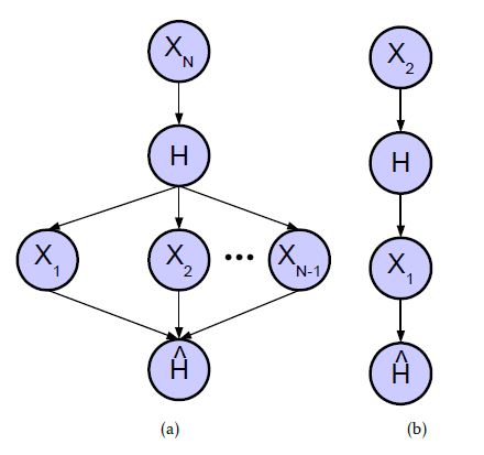Figure 6: Bayesian Network consisting of an (a) indefinite and (b) definite number of random variables Xn,1 ≤ n ≤ N.

The focus is on taking a selection decision for an arbitrary test case ti. XN now models the failure probability distribution of ti. In our previous example, as shown in Fig. 1 c), the failure probability distribution of test case t4 was calculated based on the empirically evaluated failure probabilities of test cases inside Fig. 1 c). Thus t4 was an element of C2 (N = 2), and its failure probability was modeled by X2. Analogously, X1 was defined by the empirically evaluated failure probabilities of test cases inside Fig. 1 b). In the interest of simplification, we always assume that the currently focused test case ti is an element of cluster CN and thus XN models its failure probability distribution.

Furthermore, we can calculate the dependency among Xn,1 ≤ n ≤ N. However, the Bayesian network in Fig. 6 models the statistical dependency between H and further random variables Xn,1 ≤ n ≤ N − 1. These dependencies cannot be calculated, but have to be modeled for estimating pˆFN and pˆFP .

First of all, we model the classifier Hˆ (·) as follows

 

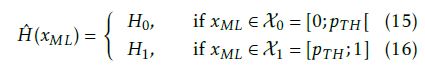
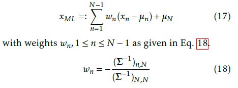
[1]) is the maximum likelihood estimation. Accordingly, the likelihood estimation is a weighted sum as given in Eq. 17

Further, pT H has to be calculated based on a precise estimation of pˆFN . Thus we derive a calculation formula for pˆFN for the case N = 2, but we will also provide a general calculation formula of pˆFN for an arbitrary number N of random variables.

6.4.1 Derivation of probability distribution functions

In the following, some probability distributions are driven that are used for estimating pˆFN . First of all, the joint pdf

 

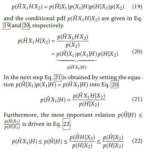
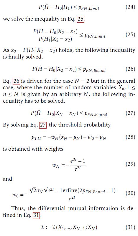
Thus, the probability calculation P (Hˆ = H0|H1) can be estimated by using the relation in Eq. 22 as given in Eq. 23.

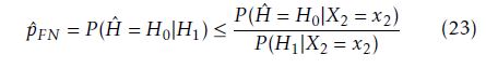
Since pˆFN cannot be directly estimated, as the conditional pdf p(Hˆ |H) is not given for performing the probability calculation P (Hˆ = H0|H1), the relation in Eq. 23 is used for estimating an upper bound for pˆFN . However, the linear classifier’s actual false-negative deselection probability would be smaller than the calculated upper bound.

Since the constraint in Eq. 24 has to be fulfilled,

 

6.4.2 Conditional Independence

We have already motivated and introduced the following dependent random variables Xn,1 ≤ n ≤ N. We have explained the fact that test case failure probabilities are correlated, since test cases are executed on the same system, and thus they show a dependent behavior.

However, the random variables Xn,1 ≤ n ≤ N are conditionally independent. This means that the information about a test case evaluation dominates such that a test case’s originally calculated failure probability becomes irrelevant after observation of its state. Accordingly, the dependency among failure probabilities vanishes after observation of test case evaluations. This means that a fail of a test case tm is actually expected based on the information about the evaluation of another test case tn and no longer on tn’s originally calculated failure probability. Thus the remaining random variables Xn,1 ≤ n ≤ N − 1 become independent of the random variable XN after observation of H’s realization (cf. Fig. 6).

6.4.3 Specificity Estimation

The specificity is given by the term 1 − pˆFP . As extensive mathematical derivations are needed for obtaining a calculation formula of pˆFP , these derivation steps are given in the appendix and in what follows here only the result is given.

Theorem 1 (False-Positive Probability Estimation). pˆFP is estimated as given in Eq. 32

 

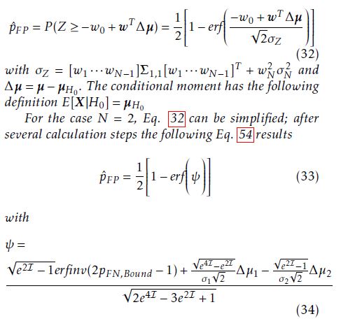
6.4.4 Small Dimension Validation

Fig. 7 shows five plots of pˆFP for different values of displacements ∆ = µn −µn,H0. Indeed, the actual value of ∆ is unknown. However, the focus is on the minimization of pˆFP . Accordingly, pˆFP decreases in each sub-figure of Fig. 7. The actual value of ∆ only determines how fast pˆFP decreases. So we can solve the optimization problem (cf. Eq. 1) by minimizing pˆFP . We considered two random variables X1 and X2, as in our example in Sec. 4 where we created two clusters. A very important factor here is the underlying strategy for clustering test cases. As the distribution of the random variables X1 and X2 is directly related to the clustering strategy the main focus is on the maximization of the differential mutual information I(X1;X2). Accordingly, I is an optimization parameter for effectively reducing pˆFP . Lastly, we chose the following values {0.01,0.05} for σ = σ1 = σ2 and selected the following displacements ∆ = α·v·10−3 with α ∈ {0;1;5;10;15} and v = [1,−1]T .

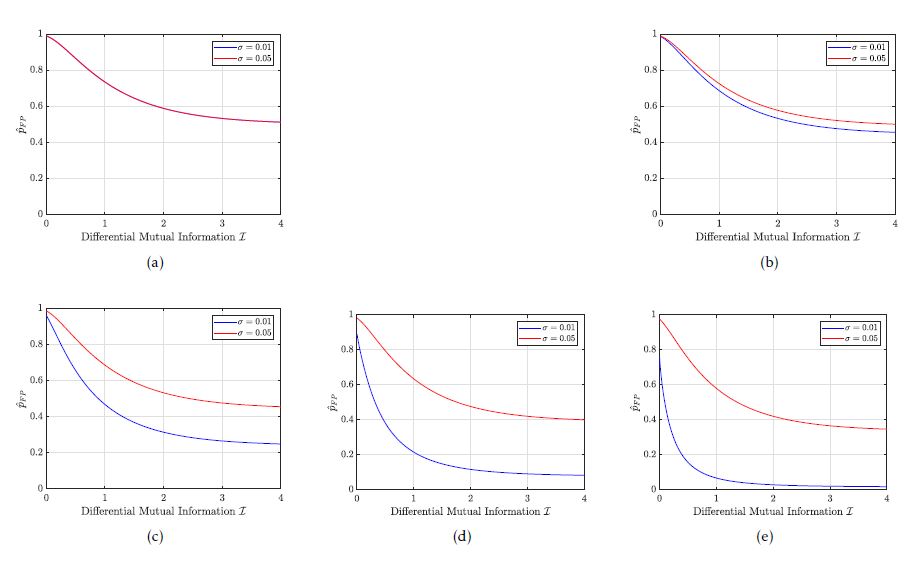Figure 7: Estimation of pˆFP for different values of ∆ and σ with ∆ = α ·v ·10−3. The value of α is 0, 1, 5, 10 and 15 in Fig. 7 a), Fig. 7 b), Fig. 7 c), Fig. 7 d) and Fig. 7 e) respectively.

7 Optimization

The first strategy is to optimize the feature selection. Optimal features are learned in an unsupervised learning session where an evolutionary optimization framework is applied to search for optimal features. The next strategy is to improve the labeling of test cases through an active learning strategy.

7.1   Evolutionary Optimization

Clustering (and sub-clustering) of test cases is performed based on features. Therefore, different clusterings for different selections of feature subsets (Φm,Φs) are possible. Accordingly, a different statistical model is obtained, as it reflects the failure frequencies in clusters. Furthermore, the differential mutual information (cf. Eq. 31) depends on the statistical dependencies and thus changes for different clusterings.

Sec. 6 proposed a calculation formula for the weights wn,0 ≤ n ≤ N, of a linear classifier. However, those formulas still depend on the differential mutual information I. A desired sensitivity has to be guaranteed, and thus the hyperplane is adjusted according to the value of I. It can be shown that for small values of I, the position of the hyperplane still guarantees a desired sensitivity but the false-positive selection probability increases. To minimize the false-positive selection probability, the differential mutual information has to be maximized, which is the final strategy for solving the constrained optimization problem (cf. Eq.1).

First, clustering depends on the history-tuples of test cases as, for example, the length of the historytuples determines the maximum number |S|K of clusters. Second, feature selection is optimized. All in all, we have summarized that K (number of considered previous regressions) is an optimization parameter and bs (for coding selected and main features) is an optimization matrix. However, this is a large-scale high dimensional optimization problem, as there exist many possible settings for K and bs. Thus, [3] and [4] suggest that the high dimensional optimization problem can be solved in a reasonable time by using evolutionary algorithms. Accordingly, an evolutionary optimization framework is applied for solving the mentioned high dimensional optimization problem. As each setting for K and bs is one possible solution for clustering test cases, which is the basis for derivation of a stochastic model, the fitness of this solution can be evaluated by calculating the extracted information I in Eq. 31. Thus, the optimal parameter and matrix setting with the best fitness will survive and will be returned by the evolutionary optimization algorithm.

Fig. 8 shows the overall flow chart of the evolutionary optimization framework. First of all, a new population consisting of several genotypes is initialized. Each genotype stands for a possible setting of K and bs . In the next step, the corresponding phenotypes of the genotypes are derived. Hence each phenotype encodes a stochastic model. Accordingly, the population is evaluated, wherein the fitness of each phenotype is calculated. However, a bad fitness is also possible due to bad statistical properties of the underlying stochastic model. This means that statistical calculations based on the stochastic model that a phenotype encodes cannot guarantee desired statistical confidence bounds. This will be explained in more detail in Sec. 8. Those phenotypes with bad fitness cannot survive and hence are eliminated.

Accordingly, remaining genotypes (phenotypes) are stochastically selected, and successively new genotypes are generated due to crossover and mutation operations. After a certain number of iterations, the phenotype with the best fitness will be selected, and this will be used in the selection algorithm. However, if the population is empty since all phenotypes were of bad fitness, then the training mode is activated, in which test cases are still executed without running the selection algorithm.

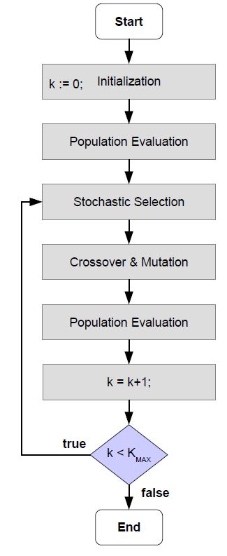Figure 8: Evolutionary Optimization Framework.

7.2   Active Learning

Our classifier’s conducted decisions can be regarded as hard or even as soft decisions. Once taken, hard decisions are never changed later on, in contrast to soft decisions. The test efficiency can be significantly increased by conducting soft decisions as opposed to hard decisions.

7.2.1 Hard Decision

[1] performs hard decisions since a selected test case is automatically executed and a once deselected test case is never selected again in the current regression test. In the following passages, the disadvantage of conducting hard decisions will be explained in detail in relation to classifier decisions.

The linear classifier’s decision depends on the current estimation of NˆFN as it calculates the allowed residual risk pFN,Limit (cf. Eq 6) of potentially taking a wrong decision. NˆFN returns the number of supposedly unrevealed system failures that would be detected by those already deselected test cases that are elements of TExec. Accordingly, the linear classifier’s decision depends on the decisions it has already taken (TExec) and hence it is memory driven.

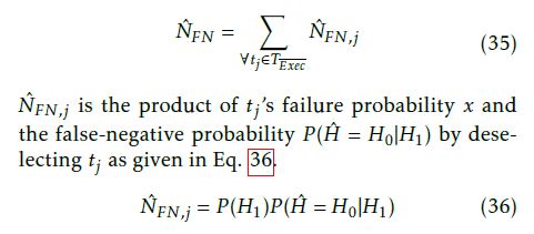
Each deselected test case tj has an individual additional contribution NˆFN,j (cf. Eq. 36) to the overall estimation NˆFN such that the relation in Eq. 35 holds.

Because of this fact, a deselection of an arbitrary test case can cause that the residual risk pFN,Limit reaches zero as NˆFN increases (cf. Eq. 6). This means that no more risk (pFN,Limit = 0) is allowed, and all remaining test cases have to be consequently selected.

Indeed, selecting test cases even if their deselection is allowed according to risk calculations is sometimes the better choice. In fact, this is the case if pFN,Limit is zero and thus it can be significantly increased by selecting and executing an already deselected test case in order to eliminate its risk. When this is done, NˆFN decreases and hence pFN,Limit increases and thus a residual risk for further deselections is obtained.

However, the amount ∆NˆFN of how much NˆFN can be decreased by selecting an arbitrary test case is significant. If later more than one test case can be deselected, and these deselected test cases add the same amount of expected unrevealed system failures ∆NˆFN to NˆFN is in fact a gain in terms of reducing the regression test effort. So the strategy is to deselect primarily those test cases with fewer failure probabilities in order to increase testing efficiency.

As a result, the regression test efficiency can be increased. Therefore, the proposed selection method [1] is extended by a soft decision methodology. So each decision for deselecting a test case is now regarded as a soft decision that might be changed later. (We note here that the other way round is impossible since an already selected test case is automatically executed on the system under test and hence deselecting it later does not make sense).

7.2.2 Soft Decision

Fig. 9 shows the logic for managing soft selection decisions: Let us assume that ti is the next test case that is analyzed by the linear classifier. If ti is deselected, then it is queued into a priority queue whereby its priority is calculated as given in Eq. 37.

prio(ti) = NˆFN,i = P (H1)P (Hˆ = H0|H1)  (37)

In the other case, if ti is selected then test cases deselected up to this point are analyzed to the end of improving the trade-off between the assumed risk and the total number of deselected test cases. As a consequence, the most probable failing test case tj is obtained by taking the peek-operation on the priority queue. The priority of ti and tj is compared, and the test case with the higher priority is selected and executed on the system under test.

If tj is executed, then it is removed from the set TExec ← TExec\tj and added into the set TExec ← TExec∪ tj. Furthermore, tj’s state is evaluated eval(tj) and accordingly the empirical failure probabilities of test cases are updated in algorithm 1. Since the calculated failure probabilities are averages of test case evaluations, the failure probabilities of those sub-clusters (see Eq. 4) have to be updated where tj is an element of them. Accordingly, the failure probabilities of ∀tk ∈ TExec are updated in algorithm 1.

Algorithm 1 Test case selection algorithm

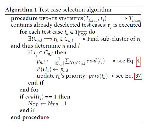
The important point is that even the failure probability of ti is computed again. In most cases, ti would be deselected. Nevertheless, it could be possible that the execution of tj has failed, such that a further system failure has been found. In such a case, even ti’s failure probability may have increased such that its deselection has to be checked again by the linear classifier.

All in all, testing efficiency can be significantly increased by performing soft selection decisions. The performance of both selection strategies (hard decision and soft decision) will be compared in Sec. 9.

8 Learning Phase

The learning phase is of essential importance due to the fact that during this phase, the system reliability is actually learned. Test case selection is a safety-critical binary classification task as probably system failures would remain undetected and hence, a corresponding quality measure of wrong decisions is required. Accordingly, risk estimations on probably undetected system failures due to deselection of test cases have to be as accurate as possible. The more the system is learned during a regression test, the more precise the risk estimations are. However, learning a system in terms of understanding its reliability is a costly process, as it requires test cases to be executed. The fundamentally important research question is how much training data is enough for safely selecting test cases with a desired sensitivity.

8.1   Statistical Sensitivity Estimation

We have already required a specific sensitivity in the constraint optimization problem (cf. Eq. 1). Accordingly, we define the following confidence level in Eq. 38, which is basically driven from the constraint of Eq. 1.

P(38)

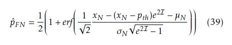
Ψ is an estimator for the number of false-negatives NˆFN = Pti∈TEXEC NˆFN,i and the bound is given as γ =NT P ·pFN,MAX             P. Ψ =1−pFN,MAX   i ψi is composed of several random variables ψi standing for the distribution of each NˆFN,i. ψi’s distribution is complex, since the individual contribution of a deselected test case ti is given by NˆFN,i = xN pˆFN where xN is ti’s failure probability and pˆFN is the corresponding estimated false-negative probability: The following theorem is already proved in [1] and gives the formula for the false-negative probability estimation.

Theorem 2 (False-Negative Probability). For a given pth the calculation formula of the false-negative probability P (Hˆ = H0|H1) has the form

where xN is the failure probability of a test case, whereas µN ,σN are parameters of the probability distribution function N (µN ,σN ).

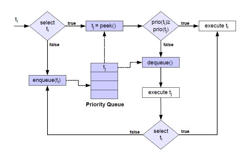Figure 9: The extended concept for conducting soft decisions

These statistics are created on the basis of sample averages, such that the consideration of sample variances becomes inevitable during the estimation of confidence intervals. For instance, the false-negative probability estimation pˆFN (see Eq. 39) is composed of the statistics xN , µN , σN and I. Therefore, its variance depends on the individual variances of each statistic, including the sample variance of xN. Especially the probability distribution of I is complex as it is nonlinearly composed of a set of multivariate distributed Gaussian random variables.

Therefore, we choose the following approach to solving Eq. 38. We simplify the definition of ψi as follows ψi = pˆFN · XN where pˆFN is assumed to be a constant value without any distribution. This step simplifies the calculation complexity of Eq. 38 significantly, as Ψ becomes simply a weighted sum of Gaussian random variables. However, the variance of pˆFN is of course relevant and should not be easily neglected. Accordingly, we require a maximum confidence interval width for pˆFN such that the estimated false-negative probability is quite accurate and hence can be assumed to be just like a constant value without any statistical deviation. We calculate the confidence interval [pˆFN ;pˆFN ] and its width δ = pˆFN − pˆFN and require a maximal confidence interval width of δmax.

The Wilson score interval [22] delivers confidence bounds for binomial proportions. Therefore, we calculate the following confidence intervals [xn ;xn ] (confidence level: 1 − α = 99%) for each failure probability estimation xn,1 ≤ n ≤ N. Each bound is consequently used for building the bounds of the composed statistics σ, Σ and I. By doing this, we obtain the following bounds: σ(b), Σ(b) and I(b) with b = {u,l}. Accordingly, we calculate pˆFN by consequently inserting the bounds σ(b), Σ(b) and I(b) for the statistics σ, Σ and I respectively.

8.2   Criteria for Training

In order to guarantee a statistical bound on the sensitivity with a 99% confidence level, the following conditions have to be checked.

1. δ ≤ δmax
2. = 99%

If both conditions are fulfilled, then these risk calculations in the selection algorithm are reasonably accurate and hence selection decisions can be performed. However, if one condition is not fulfilled then the training mode is just active, such that test cases still have to be executed.

9 Industrial Case Study

A German premium car manufacturer constitutes each regression test as being a system release test, and thus the system test takes up to several weeks according to [5]. However, a first detected system failure makes a system release impossible so optimizing the current regression for achieving high efficiency in reducing the regression effort becomes justified.

It is often the case that close to the so-called start of production (SOP) of a vehicle, many electronic control units (ECU) have only some critical spots and thus each regression test is expected to be a systemrelease test. Since many test cases pass, a lot of time is spent in observing passing test cases. Therefore, reducing the number of executed passed test cases (since a system failure is detected and a system release is no longer possible) and keeping the limited testing time back for fault-revealing test cases decreases the regression test effort significantly. In any case, a final regression test will succeed after further system updates have been conducted; this will be constituted as a final release-test that meets the high-quality standards of [5].

In our industrial case study, we applied our selection method to a production-ready controller that implements complex networked functionalities for the protection of passengers and other road users. Therefore its test effort is immense, and hence we apply our regression test selection method for accelerating its testing phase. In Fig. 10 the right-hand side of the well-known V-Model (see [23]) is shown, whereas the focus is on system testing in our case study.

A hardware-in-the-loop simulator (HiL) [24] is used for validating an ECU’s networked complex functionalities as well as its I/O-interaction and its robustness during voltage drops, as it provides an effective platform for testing complex real-time embedded systems.

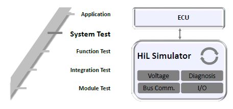Figure 10: A HiL simulator is used for performing the system test.

Further, we selected for the following test case features for training the machine learning algorithm:

• Name of verified system parts
• Name of a function for which reliability is assured
• Number of totally involved electronic control units during the testing of a networked functionality

• Error type (broken wire etc.) in hardware robustness tests
• Set of checked diagnostic trouble codes, DTCs
• Number of checked diagnostic trouble codes, DTCs

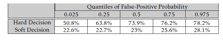
Since the quality of our selection decisions is hedged on a stochastic level, it can appear that during different runs of our selection method, a statistical deviation of the false-positive probabilities could occur. Therefore, we constitute several independent runs of a regression test, where we set pFN,MAX = 1%. The boxplots and the quantiles of the false-positive probabilities are given in Fig. 11 and in Table 4, respectively.

Fig. 11 shows the overall boxplots of the falsepositive probabilities achieved during the regression test replications. To compare the hard with the soft decision strategy we performed distinct regression test replications where we disabled and enabled the parameter for ’soft decision’, respectively.

It can be seen from Fig. 11a) and Fig. 11b) that the average false-positive probability is about 74% and 23% for hard and enabled soft decisions respectively. As already mentioned, conducting hard decisions does not allow for global optimization of the trade-off between an already assumed risk and the corresponding number of totally deselected test cases. Global optimization hence requires the analysis of all test cases deselected thus far over and over again, and, if necessary, the selection of an already deselected test case. Therefore, test cases with a higher failure probability should be considered again for eventual selection in an ongoing regression test in order to potentially deselect further less risky test cases. As a result, the regression test effort can be reduced much more by applying soft decisions.

Furthermore, the condition in Eq. 40 on the falsenegative probability pFN or on the number of actually occurring false-negatives NFN was fulfilled in all conducted regression test replications.

pFN ≤ pFN,MAX = 1% or (40)

NFN ≤ 1

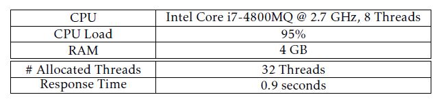
Our implemented algorithm for selecting test cases runs on a desktop CPU that is specified in Table 5. We decided to conduct a multithreaded execution of the evolutionary algorithm such that the fitness of all phenotypes in a population is computed in a multithreaded manner (in total 32 threads). Thus the average CPU load is approximately 95% and the maximum memory allocation is about 4GB. We need a mean analysis time of 0.9s for deciding whether a test case should be selected or not.

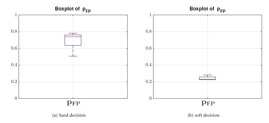Figure 11: Boxplots of false-positive probabilities in case of a) hard and b) soft decisions

Table 4: Quantiles of the false-positive probabilities in each replicated regression test

      

10 Conclusion and Future Work

We proposed a holistic optimization framework for the safety assessment of systems during regression testing. To this end, we designed a linear classifier for (de-) selecting test cases according to a classification due to a risk-associated recognition. Therefore we defined an optimization problem, since the classifier’s specificity has to be maximized whereas its sensitivity still has to exceed a certain threshold 1 − pFN,MAX. Accordingly, we developed a novel method for determining the weights of a linear classifier that solves the above optimization problem. We have theoretically shown that the classifier performance is directly interrelated with the success of selected relevant features of test cases. Lastly, we applied our method to a production-ready controller and analyzed the overall regression test effort subject to an active learning strategy. We have demonstrated that, in the regression testing of safety-critical systems, significant savings can be achieved. As feature selection is a complex task, and thus an evolutionary optimization supposedly finds local optima, more thorough research in this field may indeed allow higher-order reductions of the classifier’s false-positive selection probability.

11 Appendix

In the following, a detailed proof of Theorem 1 is given, relating to the proofs given in [1].

Proof of Theorem 1

Proof. According to [1], the maximum likelihood estimation xN,ML (abbreviated xML in the following) is given in Eq. 41.

 

 

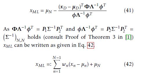
probability pth was calculated in [1] as given in Eq. 43.

 

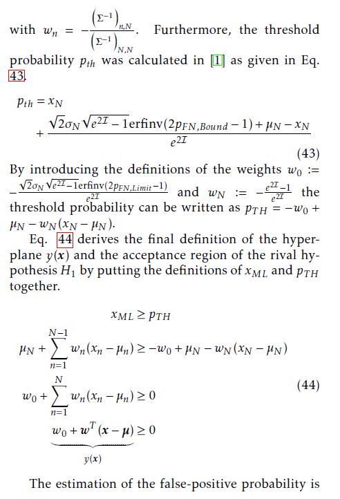
Table 5: Computational/memory requirements and algorithm performance

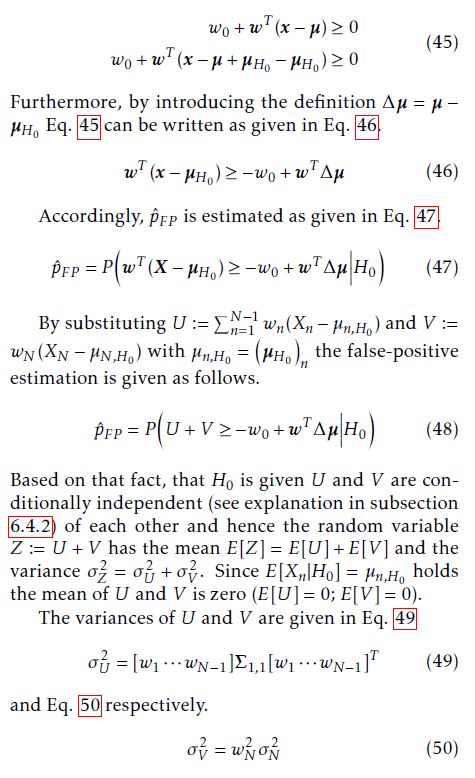
The estimation of the false-positive probability is performed by calculating pˆFP = P (Hˆ = H1|H0). However, as already explained in Sec. 6, the conditional pdf p(Hˆ |H) is not given and therefore pˆFP cannot be directly estimated. Thus, we assume that the conditional pdf p(Hˆ |H) is of a Gaussian distribution with mean E[X|H0] = µH0 and covariance matrix E[(X − µH0)(X − µH0)T |H0] = Σ. However, µH0 is an unknown parameter vector; additionally, the second-order moments are assumed to be invariant of an event H0. We will calculate pˆFP in dependency on the unknown vector µH0 and will qualitatively show that pˆFP can be minimized independently of µH0 due to an optimization strategy. In showing this, we demonstrate that the concept of our work is validated and mathematically proved.

First of all, Eq. 44 is given in Eq. 45 with an additional term.

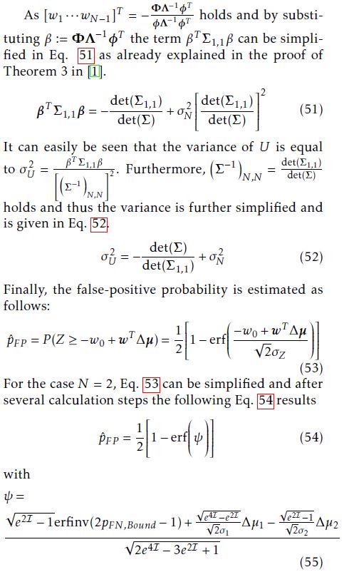
As [w1 ···wN−1]T = −ΦΛ φΛ−−11φφTT holds and by substituting β := ΦΛ−1φT the term βT Σ1,1β can be simplified in Eq. 51 as already explained in the proof of Theorem 3 in [1].

 

1. Alag¨oz, T. Herpel, and R. German, “A selection method for black box regression testing with a statistically defined quality level,” in 2017 IEEE International Conference on Software Testing, Verification and Validation (ICST), March 2017, pp. 114– 125, doi: 10.1109/ICST.2017.18.
2. B¨urger and J. Pauli, “Representation optimization with feature selection and manifold learning in a holistic classification framework,” in Proceedings of the International Conference on Pattern Recognition Applications and Methods, 2015, pp. 35–44, doi: 10.5220/0005183600350044.
3. Back, Evolutionary algorithms in theory and practice: evolution strategies, evolutionary programming, genetic algorithms. Oxford university press, 1996, doi: 10.1108/k.1998.27.8.979.4.
4. B¨urger and J. Pauli, “Understanding the interplay of simultaneous model selection and representation optimization for classification tasks,” in Proceedings of the 5th International Conference on Pattern Recognition Applications and Methods, 2016, pp. 283–290, doi: 10.5220/0005705302830290.
5. “ISO/DIS 26262-10 – Road vehicles — Functional safety,” http://www.iso.org, Tech. Rep., 2012, doi: doi:10.3403/30205385.
6. Xie and Z. Dang, “Model-checking driven black-box testing algorithms for systems with unspecified components,” CoRR, vol. cs.SE/0404037, 2004. [Online]. Available: http://arxiv.org/abs/cs.SE/0404037
7. Grosu and S. A. Smolka, Monte Carlo Model Checking. Berlin, Heidelberg: Springer Berlin Heidelberg, 2005, pp. 271–286, doi: 10.1007/978-3-540-31980-1 18. [Online]. Available: https://doi.org/10.1007/978-3-540-31980-1 18
8. Legay, B. Delahaye, and S. Bensalem, “Statistical model checking: An overview,” in International Conference on Runtime Verification. Springer, 2010, pp. 122–135, doi: 10.1007/978-3-642-16612-9 11.
9. Elkind, B. Genest, D. Peled, and H. Qu, Grey-Box Checking. Berlin, Heidelberg: Springer Berlin Heidelberg, 2006, pp. 420–435, doi: 10.1007/11888116 30. [Online]. Available: https://doi.org/10.1007/11888116 30
10. Sen, M. Viswanathan, and G. Agha, “Statistical model checking of black-box probabilistic systems,” in International Conference on Computer Aided Verification. Springer, 2004, pp. 202–215, doi: 10.1007/978-3-540-27813-9 16.
11. Peled, M. Y. Vardi, and M. Yannakakis, Black Box Checking. Boston, MA: Springer US, 1999, pp. 225–240, doi: 10.1007/978-0-387-35578-8 13. [Online]. Available: https://doi.org/10.1007/978-0-387-35578-8 13
12. Yoo and M. Harman, “Regression testing minimization, selection and prioritization: a survey,” Software Testing, Verification and Reliability, vol. 22, no. 2, pp. 67–120, 2012, doi: 10.1002/stvr.430. [Online]. Available: http://dx.doi.org/10.1002/stvr.430
13. Rothermel and M. J. Harrold, “A safe, efficient regression test selection technique,” ACM Trans. Softw. Eng. Methodol., vol. 6, no. 2, pp. 173–210, Apr. 1997, doi: 10.1145/248233.248262. [Online]. Available: http://doi.acm.org/10.1145/248233.248262
14. Orso, M. J. Harrold, D. Rosenblum, G. Rothermel, M. L. Soffa, and H. Do, “Using component metacontent to support the regression testing of component-based software,” in Proceedings IEEE International Conference on Software Maintenance. ICSM 2001, 2001, pp. 716–725, doi: 10.1109/ICSM.2001.972790.
15. -T. Cheng, L. Koc, J. Harmsen, T. Shaked, T. Chandra, H. Aradhye, G. Anderson, G. Corrado, W. Chai, M. Ispir, R. Anil, Z. Haque, L. Hong, V. Jain, X. Liu, and H. Shah, “Wide & deep learning for recommender systems,” in Proceedings of the 1st Workshop on Deep Learning for Recommender Systems, ser. DLRS 2016, vol. abs/1606.07792. New York, NY, USA: ACM, 2016, pp. 7–10, doi: 10.1145/2988450.2988454. [Online]. Available: http://doi.acm.org/10.1145/2988450.2988454
16. Langone, O. M. Agudelo, B. De Moor, and J. A. Suykens, “Incremental kernel spectral clustering for online learning of non-stationary data,” Neurocomputing, vol. 139, pp. 246–260, 2014, doi: 10.1016/j.neucom.2014.02.036 .
17. Mehrkanoon, O. M. Agudelo, and J. A. Suykens, “Incremental multi-class semi-supervised clustering regularized by kalman filtering,” Neural Networks, vol. 71, pp. 88–104, 2015, doi: 10.1016/j.neunet.2015.08.001.
18. Settles, “Active learning literature survey,” University of Wisconsin–Madison, Computer Sciences Technical Report 1648, 2009. [Online]. Available: http://axon.cs.byu.edu/ _martinez/classes/778/Papers/settles.activelearning.pdf
19. Lin, M. Mausam, and D. Weld, “Re-active learning: Active learning with relabeling,” 2016. [Online]. Available: https://www.aaai.org/ocs/index.php/AAAI/AAAI16/ paper/view/12500
20. B¨urger and J. Pauli, “Automatic representation and classifier optimization for image-based object recognition,” in VISAPP 2015 – Proceedings of the 10th International Conference on Computer Vision Theory and Applications, Volume 2, Berlin, Germany, 11-14 March, 2015., 2015, pp. 542– 550, doi: 10.5220/0005359005420550. [Online]. Available: https://doi.org/10.5220/0005359005420550
21. Handbook of Mathematics. Springer Berlin Heidelberg, 2007, doi: 1007/978-3-540-72122-2. [Online]. Available: https://doi.org/10.1007%2F978-3-540-72122-2
22. Thulin, “The cost of using exact confidence intervals for a binomial proportion,” Electron. J. Statist., vol. 8, no. 1, pp. 817–840, 2014, doi: 10.1214/14-EJS909. [Online]. Available: https://doi.org/10.1214/14-EJS909
23. Sommerville, Software Engineering: (Update) (9th Edition) (International Computer Science). Boston, MA, USA: Addison- Wesley Longman Publishing Co., Inc., 2011.
24. Schlager, Hardware-in-the-Loop Simulation: A Scalable, Component-based, Time-triggered Hardware-in-the-loop Simulation Framework. VDM Verlag Dr. M¨ uller E.K., 2013.

(Click to view)

(Click to view)