Machine Learning framework for image classification
Machine Learning framework for image classification
Volume 3, Issue 1, Page No 01-10, 2018
Author’s Name: Sehla Loussaief1,2,a), Afef Abdelkrim1,2
View Affiliations
1LA.R.A, Ecole Nationale d’Ingénieurs de Tunis, Université Tunis El Manar. BP 32, le Belvédère 1002, Tunisia
2ENICarthage, Université de Carthage, 35 rue des Entrepreneurs, Charguia II, Tunis, Tunisia
a)Author to whom correspondence should be addressed. E-mail: sehla.loussaief@gmail.com
Adv. Sci. Technol. Eng. Syst. J. 3(1), 01-10 (2018); ![]() DOI: 10.25046/aj030101
DOI: 10.25046/aj030101
Keywords: Image classification, Features extraction, Bag of Features, Class prediction accuracy, Speed Up Robust Features, Machine learning

Export Citations
Hereby in this paper, we are going to refer image classification. The main issue in image classification is features extraction and image vector representation. We expose the Bag of Features method used to find image representation. Class prediction accuracy of varying classifiers algorithms is measured on Caltech 101 images. For feature extraction functions we evaluate the use of the classical Speed Up Robust Features technique against global color feature extraction. The purpose of our work is to guess the best machine learning framework techniques to recognize the stop sign images. The trained model will be integrated into a robotic system in a future work.
Received: 17 October 2017, Accepted: 10 December 2017, Published Online: 18 January 2018
1. Introduction
This paper is an extension of work originally presented in the 7th International Conference on Sciences of Electronics, Technologies of Information and Telecommunications (SETIT), 2016. It presents the use of machine learning algorithms for image classification and exposes the Bag of Features (BoF) approach. The BoF aims at finding vector representations of input images that can be used to categorize images into a finite set of classes. This paper attempts to give a comparison between different features extraction methods and classification algorithms.
The remainder of this paper is structured as follows: Section 2 provides background information on machine learning. Section 3 gives a brief review of computer vision system, while Section 4 provides a detailed description of the Bag of Features paradigm. It also exposes the Speed Up Robust Features (SURF) detector of image Region Of Interest (ROI) and highlights the unsupervised K-Means algorithm. In section 5 we describe different learning algorithms that we will use as classifiers. Section 6 discusses experimentations carried out in order to evaluate the classification accuracy of our machine learning framework in Caltech 101 image dataset. We conclude with a discussion of open questions and current direction of image classification and feature extraction research.
2. Machine Learning Paradigm
In the past years, computer scientists developed a wide variety of algorithms particularly suited to prediction. Among these we cite: Nearest Neighbor Classification, Neural Nets, Ensembles of Trees and Support Vector Machines. These machine learning (ML) methods are easier to implement and perform better than the classical statistical approaches.
Statistical approaches to model fitting, which have been the standard for decades, start by assuming an appropriate data model witch parameters are then estimated from the data. By contrast, ML avoids starting with a data model and rather uses an algorithm to learn the relationship between the response and its predictors. The statistical approach focuses on issues such as what model will be postulated how the response is distributed, and whether observations are independent. By contrast, the ML approach assumes that the data-generating process is complex and unknown, and tries to learn the response by observing inputs and responses and finding dominant patterns [1-2].
The machine learning workflow is described in Figure 1:
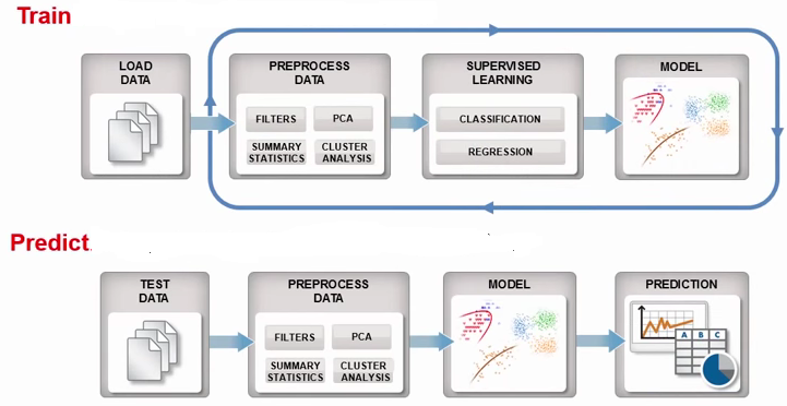 Figure 1: Machine learning workflow
Machine Learning focuses on what is being predicted, the model’s ability to predict well and how to measure prediction success.
Many fields of modern society use Machine-learning technologies: web searches, content filtering on social net-works, recommendations on e-commerce websites. Today, ML is present in consumer products such as cameras and smartphones. Machine-learning systems are used in computer vision, transcribe speech into text, match news items, posts or products with users’ interests, and select relevant results of search.
3. Computer Vision System
Computer Vision System provides algorithms, functions, and applications for designing and simulating computer vision and video processing systems. It offers image classification and retrieval [3–6], object recognition and matching [7-9], 3D scene reconstruction [10], robot localization [11], object detection and tracking and video processing. All of these processing systems rely on the presence of stable and meaningful features in the image. Thus, the most important steps in these applications are detecting and extracting the image features.
The approach consists in detecting interest regions (key-points) in each image that are covariant to a class of transformations. Then, for each detected regions, an invariant feature vector representation (i.e., descriptor) for image data around the detected key-points is built.
Two types of image features can be extracted for image content representation; namely global features and local features. Global features (e.g., color and texture) describe an image as a whole. While, local features aim to detect key-points or interest regions in an image and describe them. In this context, if the local feature algorithm detects n key-points in the image, there are n vectors describing each one’s shape, color, orientation, texture and more.
The use of global color and texture features is an efficient technic for finding similar images in a dataset. While the local
structure oriented features are adequate for object classification. It was proven that using global features cannot distinguish foreground from background of an image, and mix information from both parts together. [12].
In this work we deploy and test a machine learning based framework in object detection and recognition. We are interested on image category classification. To achieve tests we use the Calltech[1] dataset.
As the main issue in image classification is image features extraction, we use in our research the Bag of Features (BoF) techniques described in section 4.
4. Bag of Features Paradigm for Image Classification
In document classification fields (text documents), a bag of words is a sparse vector of occurrence counts of words; that is, a sparse histogram over the vocabulary. In computer vision, the bag-of-words model (BoW model) can be applied to image classification, by treating image features as words.
In computer vision, a bag of visual words is a vector of occurrence counts of a vocabulary of local image features. To encode an image using BoW model, an image can be treated as a document. Thus, “words” in images need to be defined. For this purpose, we use three steps: feature detection, feature description, and codebook generation [13-15].
4.1. Features Detection
In image processing the concept of feature detection refers to techniques that aim at abstractions of image information. Computer vision is using these extracted informations in making local decisions. Given that, a feature is defined as an “interesting” part of an image. The resulting features will be subsets of the image domain, often in the form of isolated points, continuous curves or connected regions [16].
Feature detection is a low-level image processing operation. That is, it is usually performed as the first operation on an image. It examines every pixel to see if there is a feature present at that pixel. If this is part of a larger algorithm, then the algorithm will typically only examine the image in the region of the features.
As a built-in pre-requisite to feature detection, the input image is usually smoothed by a Gaussian kernel in a scale-space representation and one or several feature images are computed, often expressed in terms of local image derivatives operations [17].
Common features detectors: Canny, Sobel, Level curve curvature, FAST, Laplacian of Gaussian, MSER, Grey-level blobs.
4.2. Features Description
After feature detection, each image is abstracted by several local patches. Feature representation methods represent the patches as numerical vectors called feature descriptors. A descriptor should have the ability to handle intensity, rotation, scale and affine variations to some extent.
One of the most famous descriptors is Scale-invariant feature transform (SIFT) [18]. SIFT converts each patch to 128-dimensional vector. After this step, each image is a collection of vectors of the same dimension (128 for SIFT), where the order of different vectors is of no importance.
4.3. Codebook Generation
Finally, the BoW model converts vector-represented patches to “codewords”, which also produces a “codebook” (word dictionary). A codewords can be considered as a representative of several similar patches.
The most used method for building a codebook is performing k-means (section 4.5) clustering over all the vectors. Codewords are then defined as the centers of the learned clusters. The number of the clusters is the codebook size (the size of the word dictionary). Thus, each patch in an image is mapped to a certain codeword through the clustering process and the image can be represented by the histogram of the codewords [19].
In image classification, an image is classified according to its visual content. The feature vector consists of SIFT/SURF features computed on a regular grid across the image and vector quantized into visual words.
The frequency of each visual word is then recorded in a histogram for each tile of a spatial tiling.
The final feature vector for the image is a concatenation of these histograms.
4.4. Speed Up Robust Features (SURF) Extraction Technique
The Speed Up Robust Features method extracts salient features and descriptors from images. This extractor is preferred over Scale-Invariant Feature Transform (SIFT) due to its concise descriptor length. The standard SIFT implementation uses a descriptor consisting of 128 floating point values.
SURF algorithm condenses this descriptor length to 64 floating point values.
It constructs a descriptor vector of length 64 using a histogram of gradient orientations in the local neighborhood around each key-point [20].
SURF considers the processing of grey-level images only, since they contain enough information to perform feature extraction and image analysis [21].
The implementation of SURF used in this paper is provided by the Matlab R2015a library.
4.5. Descriptors clustering: K-Means
Bag of Features (BoF) model is a key development in image classification using key-points and descriptors.
The descriptors extracted from the training images are grouped into N clusters of visual words using unsupervised learning algorithms such as K-means. A descriptor is categorized into its cluster centroid using an “Euclidean distance” metric. For input image, each extracted descriptor is mapped into its nearest cluster centroid.
A histogram of counts is constructed by incrementing a cluster centroid’s number of occupants each time a descriptor is placed into it. The result is that each image is represented by a histogram vector of length N. It is necessary to normalize each histogram by its L2-norm to make this procedure invariant to the number of descriptors used. Applying Laplacian smoothing to the histogram appears to improve classification results.
K-means clustering is selected over Expectation Maximization (EM) to group the descriptors into N visual words [22]. Experimental methods verify the computational efficiency of K-means as opposed to EM. Our specific application necessitates rapid training which precludes the use of the slower EM algorithm.
5. Learning and Recognition Based on BoW Models
Computer vision researchers have developed several learning methods to leverage the BoF model for image related tasks. For multiple label categorization problems, the confusion matrix can be used as an evaluation metric.
A confusion matrix is defined as a specific table layout that allows visualization of the performance of a supervised learning algorithm. Each column of the matrix represents the instances in a predicted class while each row represents the instances in an actual class (or vice-versa). The name stems from the fact that it makes it easy to see if the system is confusing two classes (i.e. commonly mislabeling one as another) [23].
In this work we investigate many supervised learning algorithms. These learning algorithms are used to classify an image using the histogram vector previously constructed in the K-means step.
5.1. Support Vector Machine
Classifying data is a common task in machine learning. A support vector machine (SVM) technic constructs a hyperplane or set of hyperplanes in a high- or infinite-dimensional space.
It can be used for classification, regression, or other tasks. A good separation is achieved by the hyperplane that has the longest distance to the nearest training-data point of any class (so-called functional margin). A larger margin induces lower generalization error of the classifier [24].
Classification of images and Hand-written character recognition can be performed using SVMs. The SVM algorithm has, also, been widely applied in the biological and other sciences.
5.2. Nearest Neighbor Classification
In pattern classification, the k-nearest neighbors (kNN) rule is the oldest. It is also considered as the simplest methods. The kNN rule classifies each unlabeled example by the majority label among its k-nearest neighbors in the training set. The distance metric used to identify nearest neighbors influences greatly its overall performance.
In the absence of prior knowledge, most kNN classifiers use simple Euclidean distances to measure the dissimilarities between examples represented as vector inputs.
Euclidean distance metrics, however, do not capitalize on any statistical regularity in the data that might be estimated from a large training set of labeled examples [25].
5.3. Boosted Regression Trees (BRT)
The BRT technique target is to improve the performance of a single model. This is achieved by fitting many models and combining them for prediction. BRT uses two algorithm categories:
- Decision tree learning algorithm which uses a decision tree as a predictive model. It maps observations about an item to conclusions about its target value. It is one of the predictive modelling approaches used in statistics, data mining and machine learning. When the target variable can take a finite set of values, the tree models are called classification trees. In these tree structures, leaves represent class labels and branches represent conjunctions of features that lead to those class labels. Decision trees where the target variable can take continuous values (typically real numbers) are called regression trees [26].
- Gradient boosting algorithm which is a machine learning technique used for regression and classification problems. It produces a prediction model in the form of an ensemble of weak prediction models, typically decision trees. It builds the model in a stage-wise fashion and it generalizes them by allowing optimization of an arbitrary differentiable loss function [27].
6. Experiments and Evaluation
This section provides an overview of different experiments that we use to evaluate the performance of our image classification machine learning framework.
We next describe the dataset used for testing followed by experimentation of SURF local features extractor. Next, we evaluate the impact of the categories number used in training on the accuracy of prediction. The last part of our work will focus on comparing the accuracy of different classifiers.
6.1. Dataset
Our results are reported on Calltech 101 image dataset to which we have added some new images of existing categories. Pictures of objects belong to 101 categories. Each category includes 40 to 800 images. The dataset was collected in September 2003 by Fei-Fei Li, Marco Andreetto, and Marc ‘Aurelio Ranzato. The size of each image is roughly 300 x 200 pixels. We are interested in stop sign category recognition.
6.2. SURF Local Feature Extractor and Descriptor
In the first part of experimentation we test the local feature extractor SURF and its robustness in matching features even after rotation and scaling image.
SURF is a scale and rotation invariant interest point detector and descriptor.
The feature finding process is usually composed of two steps; first, find the interest points in the image which might contain meaningful structures; this is usually done by comparing the Difference of Gaussian (DoG) in each location in the image under different scales. The second step is to construct the scale invariant descriptor on each interest point found in the previous step.
As first experimentation we use Matlab functionalities to test the SURF point of interest extraction function on sign stop images (Figure. 2, Figure. 3). Next we test the SURF matching features capability (Figure. 4).
6.3. Bag of Features Image Encoding
Features extracted in the first step will be used to represent each image category. To do that, the K-means clustering is used to reduce the number of features for proper classification. Only strongest features are considered. The encode approach is then applied. Thus, each image of the dataset is encoded into a vector feature using BoF.
The feature vector of an image represents the histogram of visual word occurrences contained in it. This histogram considered a basis for training the classifier. Figure 5 represents encoding results for some stop sign images.
6.4. Classifier Training Process
The encoded training images from each category are fed into a classifier training process to generate a predictive model.
Figure 6 illustrates the steps of the approach used in our image classification framework.
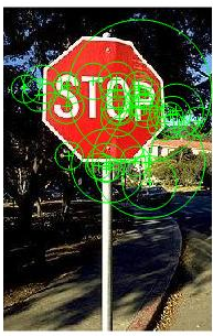 Figure 2: SURF Features Detection Figure 2: SURF Features Detection |
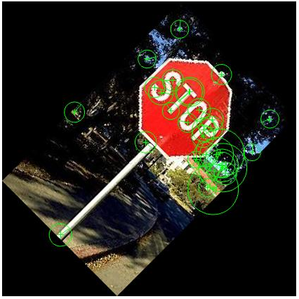 Figure 3: SURF Features Detection in rotated (30°) and scaled (1.5) image Figure 3: SURF Features Detection in rotated (30°) and scaled (1.5) image |
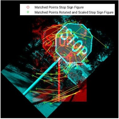 Figure 4: SURF point matching capabilities Figure 4: SURF point matching capabilities |
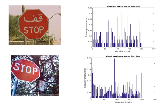 Figure 5: Histogram of visual words occurrences on stop sign images
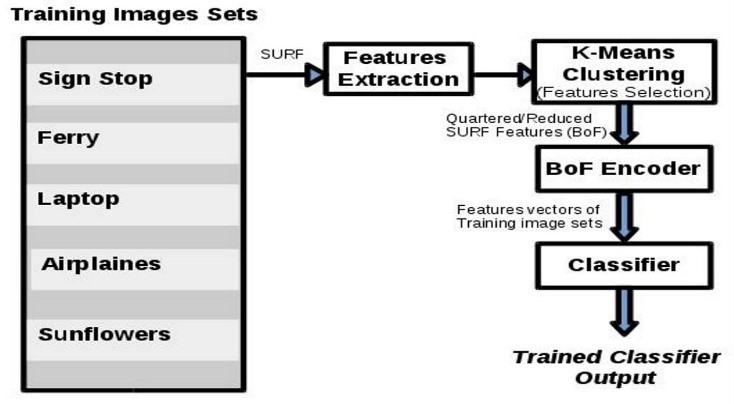 Figure 6: Image classification process
In this section, we are interested in measuring the average accuracy and the confusion matrix of the classifying process through different experimentations. For this purpose, we use some image categories from the Calltech101dataset. These classes are described in Table 1.
Experiment 1: Two categories classification accuracy measurement using SURF extractor
The Linear SVM classifier is used to generate a prediction model based on two image classes. During the training process we use 70% of the whole image dataset. The remaining images are included in the test dataset and used in the prediction assessment step. Measurements report that the achieved prediction average accuracy is 0.99 (Table 2).
Experiment 2: Three categories classification accuracy measurement using SURF extractor
During this experiment we fix the classifier to Linear SVM and the number of image categories to three. Image dataset is split to training dataset (70% of image dataset) and test dataset.
Measurements show that the achieved prediction average accuracy is 0.89 (Table 3).
Experiment 3: Four categories classification accuracy measurement using SURF extractor
For this prediction accuracy evaluation, we use the Linear SVM classifier and increase the image categories to four in order to measure the average accuracy of the classification process. It is reported that this achieved average accuracy is 0.88 (Table4).
Experiment 4: Five categories classification accuracy measurement using SURF extractor.
The Linear SVM classifier is used to classify between five image categories. It is reported that the achieved prediction average accuracy is 0.78 (Table 5).
As shown in Figure 7, we notice that the average accuracy of the classifier is influenced by the number of categories in training dataset. This metric is lower when the numbers of sets increase.
Experiment 5: Three categories classification accuracy measurement using a custom features extraction function: Color extractor.
During this experiment we use the Linear SVM as classifier and fix the number of image categories to three. For image vector representation we use a global features extractor instead of the SURF technique.
It is reported that the prediction average accuracy is 0.76 (Table 6) which is lower than the one achieved during Experiment 2.
Table 1: Image Dataset categories
| Set category |
Stop Sign Images |
Ferry Images |
Laptop images |
Airplanes images |
Sunflower images |
| Set size | 69 | 67 | 81 | 800 | 85 |
Table 2: Learning confusion matrix with two image categories
| Predicted | ||
| Known | Stop Sign | Ferry |
| Stop Sign | 0.98 | 0.02 |
| Ferry | 0.00 | 1.00 |
Table 3: Learning confusion matrix with three image categories
| Predicted | |||
| Known | Stop Sign | Laptop | Ferry |
| Stop Sign | 0.93 | 0.04 | 0.03 |
| Laptop | 0.02 | 0.77 | 0.21 |
| Ferry | 0.00 | 0.02 | 0.98 |
Table 4: Learning confusion matrix with four image categories
| Predicted | ||||||
| Known | Stop Sign | Laptop | Ferry | Airplanes | ||
| Stop Sign | 0.95 | 0.05 | 0.00 | 0.00 | ||
| Laptop | 0.00 | 0.90 | 0.10 | 0.00 | ||
| Ferry | 0.00 | 0.00 | 0.85 | 0.15 | ||
| Airplanes | 0.00 | 0.05 | 0.10 | 0.85 | ||
Table 5: Learning confusion matrix with five image categories
| Predicted | ||||||
| Known | Stop Sign | Laptop | Ferry | Airplanes | Sunflowers | |
| Stop Sign | 0.97 | 0.00 | 0.00 | 0.00 | 0.03 | |
| Laptop | 0.07 | 0.49 | 0.14 | 0.10 | 0.20 | |
| Ferry | 0.02 | 0.00 | 0.76 | 0.17 | 0.05 | |
| Airplanes | 0.00 | 0.04 | 0.20 | 0.75 | 0.01 | |
| Sunflowers | 0.00 | 0.00 | 0.02 | 0.00 | 0.98 | |
Table 6: Learning confusion matrix using global color features extractor
| Predicted | |||
| Known | Stop Sign | Laptop | Ferry |
| Stop Sign | 0.84 | 0.04 | 0.12 |
| Laptop | 0.10 | 0.67 | 0.23 |
| Ferry | 0.02 | 0.22 | 0.76 |
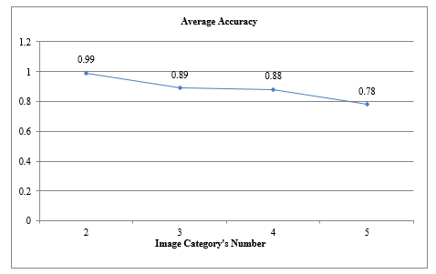 Figure: 7: Average accuracy variation based on image category’s number
We notice that in our approach is better to use a Local feature extractor (SURF) than a global features extractor. This result is expected as the global features extraction technique is better with scene categorization and examination of surrounding environment (an image may be categorized as an office, forest, sea or street image) and not for object classification [28].
Experiment 6: Evaluating image category classification using different training learner.
We next fix the number of categories to 4, the features extraction technique to SURF and evaluate prediction models on varying the classifier algorithm. In each test we calculate the confusion matrix and average accuracy on validation dataset. We use 70% of data as a training set. The application trains the model on training set and assesses the performance with the validation set. Tables 7 to Table 14 illustrate the obtained confusion matrix.
We then generate the histogram (Figure 8) of the average accuracy based on the training classifier. For this purpose we varied the classifier trainer from SVM, KNN and ensemble classifier categories.
Measurements show that the image classification process performs better when we use a likehood SVM. It’s reported that the Cubic SVM yields average accuracy which reaches 90%. The KNN techniques offer an average accuracy around 65%. Among the ensemble classifier trainers (2 last tested algorithms) the bagged trees achieves the best accuracy.
|
Table 7: Confusion matrix for Linear SVM
|
Table 8: Confusion matrix for Fine Gaussian SVM
|
|||||||||||||||||||||||||||||||||||||||||||||||||||||||||||||||||||
|
Table 9: Confusion matrix for Quadratic SVM
|
Table 10: Confusion matrix for Cubic SVM
|
|||||||||||||||||||||||||||||||||||||||||||||||||||||||||||||||||||
|
Table 11: Confusion matrix for Fine KNN
|
Table 12: Confusion matrix for Weighted KNN
|
|||||||||||||||||||||||||||||||||||||||||||||||||||||||||||||||||||
|
Table 13: Confusion matrix for Boosted Trees
|
Table 14: Confusion matrix for Bagged Trees
|
|||||||||||||||||||||||||||||||||||||||||||||||||||||||||||||||||||
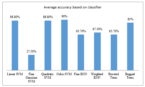 Figure 8: Average accuracy based on the learning classifier
7. Conclusion
In this paper, we related the different techniques and algorithms used in our machine learning framework for image classification. We presented machine learning state-of-the-art applied to image classification. We introduced the Bag of Features paradigm used for input image encoding and highlighted the SURF as its technique for image features extraction. Through experimentations we proofed that using SURF local feature extractor method for image vector representation and SVM (cubic SVM) training classifier performs best prediction average accuracy. In test scenarios we focused on stop sign image as we project to apply the trained classifier in a robotic system.
- Breiman, Statistical modeling: the two cultures. Statistical Science, 16, 199–215, 2001.
- Ramanathan, L. Pullum, H. Faraz, C. Dwaipayan, J. K. Sumit, “Integrating symbolic and statistical methods for testing intelligent systems: Applications to machine learning and computer vision” in Design, Automation & Test in Europe Conference & Exhibition (DATE), Dresden, Germany, 2016.
- Liu, X. Bai, Discriminative features for image classification and retrieval. Pattern Recognition. Lett. 33(6), 744–751, 2012.
- David Jardim; Luís Nunes; Miguel Dias, “Human Activity Recognition from automatically labeled data in RGB-D videos” in 8th Computer Science and Electronic Engineering (CEEC), Colchester, UK ,2016. https://doi.org/10.1109/CEEC.2016.7835894
- Stöttinger, A. Hanbury,N. Sebe, T. Gevers, “Sparse color interest points for image retrieval and object categorization” IEEE Trans. Image Process. 21(5), 2681–2691, 2012. https://doi.org/ 10.1109/TIP.2012.2186143
- Wang,Y. Li, Y. Zhang,C. Wang, H. Xie, G. Chen, X. Gao, Bag-of-features based medical image retrieval via multiple assignment and visual words weighting. IEEE Trans. Med. Imaging 30(11), 1996–2011, 2011. https://doi.org/10.1109/TMI.2011.2161673
- Miksik, K. Mikolajczyk, “Evaluation of local detectors and descriptors for fast feature matching” in International Conference on Pattern Recognition (ICPR 2012), pp. 2681–2684. Tsukuba, Japan, 2012.
- Kim, H. Yoo, K. Sohn, Exact order based feature descriptor for illumination robust image matching. Pattern Recognition. 46(12), 3268–3278, 2013.
- T T Dhivyaprabha, P. Subashini, M. Krishnaveni, “Computational intelligence based machine learning methods for rule-based reasoning in computer vision applications”, in IEEE Symposium Series on Computational Intelligence (SSCI), Athens, Greece, 2016. https://doi.org/10.1109/SSCI.2016.7850050
- Moreels, P. Perona, “Evaluation of features detectors and descriptors based on 3D objects”, in Tenth IEEE International Conference on Computer Vision (ICCV’05) Volume 1, Beijing, China, 2005. https://doi.org/10.1109/ICCV.2005.89
- M. Campos, L. Correia, J.M.F. Calado, Robot visual localization through local feature fusion: an evaluation of multiple classifiers combination approaches. J. Intell. Rob. Syst. 77(2), 377–390, 2015.
- Zhang, Q. Tian, Q. Huang, W. Gao, Y. Rui, “USB: ultrashort binary descriptor for fast visual matching and retrieval”,in IEEE Transactions on Image Processing, 2014. https://doi.org/ 10.1109/TIP.2014.2330794
- Fei-Fei ,P. Perona, “A Bayesian Hierarchical Model for Learning Natural Scene Categories”, in 2005 IEEE Computer Society Conference on Computer Vision and Pattern Recognition (CVPR’05) 2: 524. doi:10.1109/CVPR.2005.16. ISBN 0-7695-2372-2, 2005. https://doi.org/10.1109/CVPR.2005.16
- Jyothy, S. Martish, M. Leena, “Bag of feature approach for vehicle classification in heterogeneous traffic”, in IEEE International Conference on Signal Processing, Informatics, Communication and Energy Systems (SPICES), Kollam, India, 2017. https://doi.org/10.1109/SPICES.2017.8091346
- Zhang; A. P. Leung, “A Novel approach to dictionary learning for the bag-of-features model”, in International Conference on Wavelet Analysis and Pattern Recognition (ICWAPR), Ningbo, China, 2017. https://doi.org/10.1109/ICWAPR.2017.8076672
- Lindeberg, Scale selection, Computer Vision: A Reference Guide, (K. Ikeuchi, ed.), Springer, pages 701-713, 2014.
- Rosten, T. Drummond, Machine learning for high-speed corner detection. European Conference on Computer Vision. Springer. pp. 430–443. https://doi.org/10.1007/11744023_34, 2006.
- Vidal-Naquet, Ullman, “Object recognition with informative features and linear classification” in Proceedings Ninth IEEE International Conference on Computer Vision (PDF),Nice, France, 2003. https://doi.org/ 10.1109/ICCV.2003.1238356
- Cuingnet, C. Rosso, M. Chupin, S. Lehéricy, D. Dormont, H. Benali, Y. Samson, O. Colliot, Spatial regularization of SVM for the detection of diffusion alterations associated with stroke outcome, Medical Image Analysis, 15 (5): 729–737, 2011.
- Lowe, Towards a computational model for object recognition in IT cortex. Proc. Biologically Motivated Computer Vision, pages 2031, 2000.
- Mark, S. Nixon Alberto, Feature Extraction and Image Processing, Elsevier Ltd, ISBN: 978-0-12372-538-7, 2008.
- G Lowe, Distinctive image features from scale-invariant keypoints. IJCV, 60(2):91–110, 2004.
- W David, Evaluation: From Precision, Recall and F-Measure to ROC, Informedness, Markedness & Correlation (PDF). Journal of Machine Learning Technologies 2 (1): 37–63, 2011.
- Piyush, Hyperplane based Classification: Perceptron and (Intro to) Support Vector Machines, CS5350/6350: Machine Learning September 8, 2011.
- Domeniconi, D. Gunopulos, J. Peng, “Large margin nearest neighbor classifiers” in IEEE Transactions on Neural Networks, 2005. https://doi.org/10.1109/TNN.2005.849821
- Rokach,O. Maimon, Data mining with decision trees: theory and applications. World Scientific Pub Co Inc. ISBN 978-9812771711, 2008.
- H Friedman, Greedy Function Approximation: A Gradient Boosting Machine, 1999.
- Jinyi, L. Wei, C. Chen, D. Qian, Scene classification using local and global features with collaborative representation fusion; Information Sciences 348, 2016.