1. Introduction

This paper is an extension of work originally presented in PEDG conference [1].

The use of induction generators in generation systems is usual in wind plants [2-4] or eventually in small hydroelectric generation units [5]. Otherwise, from studies started in [1], it is shown a new knowledge border which consider the use of IG in parallel of SG in an isolated electric system. The first results and behavior of this kind of generation system were shown in [1] and are followed by this current article with original and deeper analysis.

Then, this work is composed of analysis over an expanded system that includes an induction motor, a resistive load, an autotransformer connected to a diodes bridge to feed the DCM_IG armature and then permits to increase manually the output electric power limits if compared to flux variation method (3) presented in [1]. Therefore, this article shows the IG supplying more active power and the induction motor inserted in experiment what enables a novel analysis of the system behavior.

This paper presents results that show additional remarkable characteristics by operation in parallel mode among one SG and one IG. Some characteristics, such as reduced weight and size, easier maintenance, and shorter manufacturing and delivery time are more associated with induction generators and are relevant to oil platforms or offshore installation concerns. Besides, it has absence of dc supply for excitation and better transient performances [5].

One of the potential motivation for this study is to develop a potential alternative capable of optimizing the main electric system currently adopted in oil platforms and floating production storage and offloading (FPSO) ships to become cheaper, simpler, lighter, and more efficient.

The potential application of this study is the replacement of one or two synchronous generators by one or two induction generators in oil offshore platforms or FPSO. A typical offshore electric system uses three or four turbo-generators in 13800 V, 60 Hz, driven by dual fuel (fuel gas or diesel oil) turbines. In typical operation, three main turbo-generators operate and can supply all unit consumers with the fourth in standby. During the peaks of load, the fourth main turbo-generator may be required to meet the demand. Therefore, the whole electric system shall be suitable for this operational condition.

Therefore, the study target is to analyze various aspects of topology and operating involving an induction generator in parallel with a synchronous generator for application in an isolated electric system, and to establish the operational viability, advantages and challenges.

2. Isolated Electric System

The isolated electric system was sized as shown in the following equations and data. The automatic controls of the system consist of a voltage control loop and a speed control loop. Both are inserted in the SG scheme as shown in Figure 5 and Figure 6. The dataplates of the principal equipment are shown in Tables 1 to 6.

The parameterization used in both electronic control boards is indicated in [1], except for the references of voltage and speed for each of the control loops which are respectively 65.5 and 65.2 as shown in Figure 9.

2.1.  Dataplate

In tables 1 to 4 are shown the main equipment’s dataplates and the tables 5 to 6 are shown the load’s dataplates used in the experiments along this work.

Table 1: DMC_IG Dataplate

Direct Current Motor IG
220 V	7.72 A	1.7 kW	1500 rpm	600 mAfieldmax

Table 2: DMC_SG Dataplate

Direct Current Motor SG
220 V	9.1 A	2.0 kW	1800 rpm	600 mAfieldmax

Table 3: IG Dataplate

Induction Generator (IG)
220 V	7.5 A	1.86 kW	1410 rpm	0.8 PF	50 Hz

Table 4: SG Dataplate

Synchronous Generator (SG)
230 V	5.0 A	2.0 kVA	1800 rpm	0.8 PF	60 Hz
Vfield: 220 V			Ifieldmax: 600 mA

Table 5: Load Dataplate

Resistive Load
Load 1 (kW)	Load 2 (kW)	Load 3 (kW)
2/3	2/3	2/3

Table 6: Load, Induction Motor Dataplate

Induction Motor
0.37 kW	1715 rpm	Cos ϕ: 0.71	60 Hz

2.2.  Equations – Part I

Follow the main equations for analysis comprehension and to establish a studies base:

• Direct Current Motor

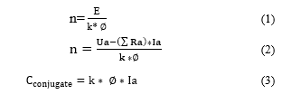• Synchronous Generator

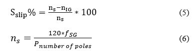
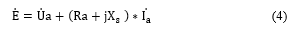• Induction Generator

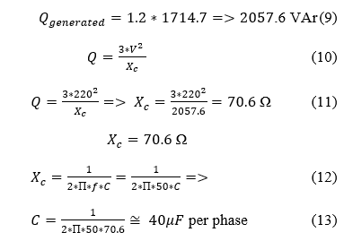
2.3.  Capacitor Bank Sizing

As informed at the IG dataplate

The reactive power is calculated to attend the reactive demand of the Induction Machine:

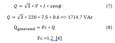
For the machine coupled at a resistive load which requires 7.5A, it is necessary for the reactive power generation to be approximately 2057.6 VAr as demonstrated below.

2.4.  Resistive Divider Sizing:

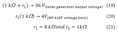
• Field Control Loop Resistive Divider as in Figure 5 and Figure 6.

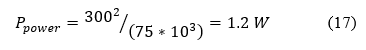
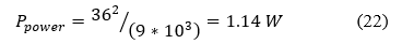
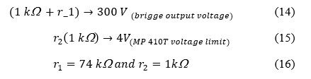• Resistor Power Sizing:

• The resistors that were selected based on the sized resistor, were:

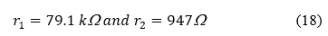• Speed Control Loop Resistive Divisor as in Figure 5 and Figure 6.

• Resistor Power sizing:

• The resistors chosen, based on the sized resistor, were

2.5.  Equations – Port II

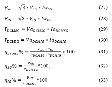
Follow the system equations base to calculate the power and efficiencies shown in Table 7 and Table 8 for each generator and entire group of machines.

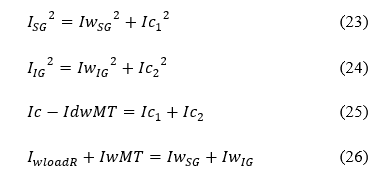As I_SG, I_IG, IC and I_wloadR are measured values, shown in Table 7 and Table 8, IdwMT(Motor’s reactive current) and IwMT(Motor’s active current) are values calculated in appendix 1. Then, the system has 4 four variables and 4-four equations. Then, for each scenario, the four variables , ,  and  were calculated by Matlab software and are shown in Table 7 and Table 8.

The entire group efficiency and the efficiency of each subgroup were calculated based on PIG, PSG, PDCMSG, and PDCMIG, as follows:

2.6.  Equations – Part III

The equations e calculus used to determined the IM parameters and IM equivalent circuit as primary, secondary impedances and currents, including IM currents showed in Table 8 are calculated in item 5 of appendix 1.

2.7.  The Experiment and Schemes

The experiment was mounted in the laboratory as shown in Figure 1 and Figure 2. The detailed circuit is shown in Figure 6. Figure 2 shows another experiment view, including the taco generator and its connections. The detailed circuit is shown in Figure 6. Figure 3 shows the typical connections of both circuit board MP 410T which are implemented in this experiment for the voltage loop and speed loop. They are also indicated in Figure 5 and Figure 6.

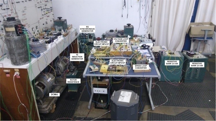Figure 1 Laboratory assembly

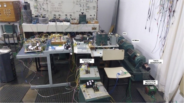Figure 2 Another view of laboratory assembly

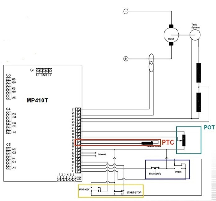Figure 3. Connections arrangement of MP410T and devices

Figure 4 shows the 1B6C configuration used for the two thyristor converter bridges which were used in the control loops.

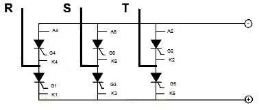Figure 4. Converters configuration used in voltage and speed loops

As seen in [1], the power from IG, PIG, was limited because the I_fDCMIG reached the maximum viable value in accordance with DCM_IG current specifications. This limited speed from DCM_IG was a challenge because it was not showing a representative contribution from PIG. It was necessary to elevate the DCM_IG speed, n_IG.

Then, the methodology consists of implementing the comparative analysis of the power and efficiencies, starting with an analysis between the PIG from the scheme in [1] and PIG from the scheme in Figure 5 and Figure 6, covering the scenarios shown in Table 7 related to Figure 5 and Table 8 related to Figure 6. Finally, a comparative efficiency analysis was conducted for two subgroups, one composed of IG and DCM_IG and the other composed of SG and DCM_SG in scenarios related to the scheme in [1] and the schemes in Figure 5 related to Table 7 and Figure 6 related to Table 8.

Thus, the increase of DCM_IG speed, increase of PIG contributions and improvement of IG subgroup efficiencies are shown in results.

Figure 6 shows the scheme implemented in the laboratory to overcome the challenge related to limitation of IG speed [1] and bring the experiment closer to actual offshore conditions, taking into advantages of IG power capacity. It was used as an autotranformer connect to a diodes bridge to vary the voltage applied on the DCM_IG armature circuit and obtain a higher speed and PIG.

2.8.  Voltage and Speed Control Loops

The Figure 7 and Figure 8 show the closed control loop used to control the SG speed and voltage via circuit boards.

Figure 9 (a) and Figure 9 (b) show the circuit boards with the respective working point or reference points defined during parameterization for the speed control loop, 65.2 and the voltage control loop, 65.5.

As [1], the master and slave behavior were verified by the generators, considering that SG is the master and IG is the slave. The frequency and voltage are determined by SG, while active power consumed at load is controlled by IG.

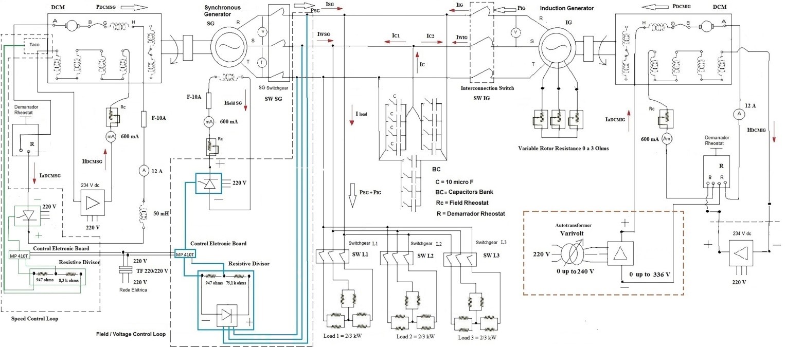Figure 5 Synchronous generator in parallel with induction generator and its dc motor_ 234 Vdc steady source for DCM_IG

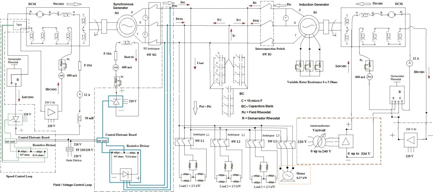Figure 6: Synchronous generator in parallel with induction generator and its dc Motors _ Vdc variable source for DCM_IG

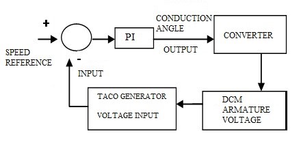Figure 7. Speed Control Loop

Note: For both regulators, the proportional gain P was experimentally set at 0,010 and, in the same manner, the time constant was set at 0,04 s as in [1].

3. Experiment Data and Results

3.1.  Experiment Data

The experimental data obtained in the laboratory are shown in Table 7 and Table 8. The Table 7 is referred to scheme in Figure 5 and Table 8 is referred to scheme in Figure 6. The unique difference is the presence of IM as additional load presented in Figure 6 scheme. Then, the Table 7 and Table 8 shows the data obtained from the scheme shown respectively in Figure 5 and Figure 6 which are similar to scheme shown in [1], except for the presence of an autotransformer in the DCM_IG field circuit for Figure 5 and Figure 6 and an IM as additional load in Figure 6.

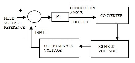Figure 8. Field voltage control loop

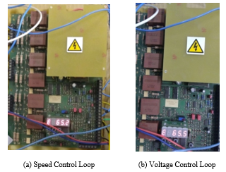Figure 9. Circuit boards MP410T used to implement the control loops

The autotransformer is responsible for applying a voltage range directly on the DCM_IG armature to obtain a larger speed range of the DCM_IG and to push more power to the IG, keeping the DCM_IG parameters into the rated values. Hence, the elevation of IG speed and power depend on just V_aDCMIG, it means this method is different from the scheme presented in [1] that depends on the DCM_IG field flux. Both V_aDCMIG and the DCM_IG field flux are adjusted manually. In summary, the [1] shows the data obtained from the scheme that has the 234Vdc steady source, Table 7 and Table 8 shows the data obtained from the schemes shown in Figure 5 and Figure 6, that has an autotransformer and a diodes bridge as substitute of the 234 Vdc steady source.

The data presented in Table 8 related to Figure 6 system performance results are compared to data obtained from Table 7 related to scheme in Figure 5 and also compared to data obtained from [1]. The scheme in Figure 5 and Table 7 shows the performance of the isolated electric system that considers the voltage application range on the DCM_IG armature by an autotransformer and an diodes bridge. The scheme in Figure 6 and Table 8 shows the performance of the isolated electric system that considers the same scheme presented in Figure 5 added by a induction motor, IM, as an additional load.

4. Results

The results and comparative analysis from experiments shown in Figure 5, Figure 6 and the results obtained in [1] are presented in the following.

The results show graphs and analysis of system configurations presented in Figure 5 and Figure 6, data obtained in [1] and analysis of contribution from each generator for each arrange of load, that, in this case, is ether just resistive banks or resistive banks added with an induction motor IM. It is noted that for all graphs obtained from [1] is related to a set system frequency of 55 Hz.

Table 7: Operational Scenarios in Controlled Mode and load being resistors bank

	SG and IG in parallel mode and no load. 40 µF / phase	SG and IG in parallel mode and load in. 40 µF /phase	SG and IG in parallel mode and load in. 40 µF /phase	SG and IG in parallel mode and load in. 40 µF /phase	SG and IG in parallel mode and load in . 40 µF /phase	SG and IG in parallel mode and load in. 40 µF /phase	SG and IG in parallel mode and load in. 40 µF /phase	SG alone and load in. 40 µF /phase	SG alone and no load. 30 µF /phase
Results	Scenario 1B	Scenario 2B	Scenario 3B	Scenario 4B	Scenario 5B	Scenario 6B	Scenario 7B	Scenario 8B	Scenario 9B
V S G       (V)	220.0	220.0	220.0	220.0	220.0	220.0	220.0	220.0	220.0
f S G     (Hz)	60	60	60	60	60	60	60,0	60,0	60,0
I fieldSG   (mA)	190	320	300	300	320	350	370	340	100
VaDCMSG   (V)	272.9	275.0	276.2	276.8	277.5	278.0	280.7	278.5	270.0
IaDCMSG    (A)	2.0	2.5	3.8	4.7	6.2	7.4	9.5	10.6	2.0
IfDCMSG  (mA)	510.0	530.0	520.0	520.0	515.0	510.0	515.0	515.0	515.0
V IG    (V)	220.0	220.0	220.0	220.0	220.0	220.0	220.0	n.a.	n.a.
fIG     (Hz)	60	60	60	60	60	60	60	n.a.	n.a.
n I G      (rpm)	1793	1896	1878	1857	1848	1821	1794	n.a.	n.a.
VaDCMIG   (V)	291.3	323.6	316.7	308.3	301.3	293.0	284.1	n.a.	n.a.
I aDCM IG   (A)	0.5	8.0	7.0	6.0	4.7	3.5	2.0	n.a.	n.a.
IfDCMI G  (mA)	330.0	330.0	330.0	330.0	330.0	330.0	330.0	n.a.	n.a.
IwloadR   (A)	0.0	5.0	5.0	5.0	5.0	5.0	5.0	5.0	0.0
IIG        (A)	2.4	5.8	5.1	4.4	3.7	2.9	2.4	0.0	0.0
ISG        (A)	2.9	1.5	2.0	2.8	3.6	4.5	5.6	7.4	4.0
IC         (A)	5.4	5.4	5.4	5.4	5.4	5.4	5.4	5.4	4.0
IWSG    (A)	0.0	1.05	1.48	1.97	2.47	3.32	4.65	5.03	0.0
IC1        (A)	2.94	1.13	1.60	2.13	2.66	3.03	3.13	5.40	4.0
IC2        (A)	2.45	4.26	3.80	3.27	2.74	2.37	2.27	0.0	0.0
IWIG      (A)	0.0	3.95	3.51	3.03	2.53	1.68	0.35	0.0	0.0
PSG   (W)	0.0	400.5	565.5	750.0	939.8	1266.6	1770.1	1915.8	0.0
PIG    (W)	0.0	1504.8	1335.8	1155.3	965.5	638.67	135.17	0.0	0.0
PDCMSG  (W)	545.8	687.5	1049.6	1301.0	1665.0	2057.2	2666.7	2962.7	543.4
PDCMIG   (W)	145.7	2588.8	2216.9	1849.8	1416.1	1025.5	568.2	0	0.0
ηGROUP   (%)	0.0	58.15	58.33	60.47	61.84	61.80	58.89	64.66	0.0
ηSG       (%)	0.0	58.25	53.88	57.65	56.44	61.57	66.38	64.66	0.0
ηIG       (%)	0.0	58.12	60.43	62.45	68.18	62.28	23.79	n.a.	n.a.

                Obs.:        1- Italic and bold text: calculated values by equations 23 to 33

                                2- Frequency was chosen based on the average between the SG and IG rated frequency

                                3- n.a: not applicable

Table 8: Operational Scenarios in Controlled Mode and load being resistors bank and induction motor

	SG and IG in parallel mode and no load. 40 µF / phase	SG and IG in parallel mode and load in. 40 µF /phase	SG and IG in parallel mode and load in. 40 µF /phase	SG and IG in parallel mode and load in. 40 µF /phase	SG and IG in parallel mode and load in. 40 µF /phase	SG and IG in parallel mode and load in. 40 µF /phase	SG and IG in parallel mode and load in. 40 µF /phase	SG alone and load in. 40 µF /phase	SG alone and no load. 30 µF /phase
Results	Scenario 1C	Scenario 2C	Scenario 3C	Scenario 4C	Scenario 5C	Scenario 6C	Scenario 7C	Scenario 8C	Scenario 9C
V S G      (V)	220.0	220.0	220.0	220.0	220.0	220.0	220.0	220	220.0
f S G     (Hz)	60	60	60	60	60	60	60	60	60
I fieldSG    (mA)	170	420	410	400	400	430	475	390	100
VaDCMSG   (V)	278.9	277.0	277.5	280.5	281.0	281.1	282.9	279.2	271.7
IaDCMSG    (A)	2.0	2.9	4.0	5.0	6,3	7,6	9,6	10,5	2,0
IfDCMSG  (mA)	530.0	530.0	530.0	530.0	530.0	520.0	520.0	520.0	515.0
V IG     (V)	220.0	220.0	220.0	220.0	220.0	220.0	220.0	0.0	n.a.
fIG      (Hz)	60	60	60	60	60	60	60	0.0	n.a.
n I G      (rpm)	1803	1893	1868	1857	1843	1821	1793	0.0	n.a.
VaDCMIG    (V)	288.9	330.0	318.0	310.0	302.3	295.2	285.9	0.0	n.a.
I aDCMIG    (A)	1.0	8.0	7.0	6.0	4.7	3.5	2.0	0.0	n.a.
IfDCMIG   (mA)	330.0	330.0	330.0	330.0	330.0	330.0	330.0	0.0	n.a.
IwloadR   (A)	0.0	5.0	5.0	5.0	5.0	5.0	5.0	5.0	0.0
IwMT      (A)	0.0	0.2	0.2	0.2	0.2	0.2	0.2	0.2	0.0
IdwMT        (A)	0.0	1.23	1.23	1.23	1.23	1.23	1.23	1.23	0.0
IIG          (A)	2,3	6,0	5,0	4,4	3,6	2,9	2,3	0.0	0.0
ISG          (A)	2.8	0.7	1.6	2.3	3.3	4.1	5.3	6.7	4.0
IC           (A)	5.4	5.4	5.4	5.4	5.4	5.4	5.4	5.4	4.0
IWSG      (A)	0.0	0.65	1.29	1.99	3.04	3.74	4.95	5.23	0.0
IC1          (A)	2.94	0.28	1.03	1.17	1.29	1.66	1.88	4.2	4.0
IC2          (A)	2.46	3.91	3.14	3.00	2.88	2.51	2.29	0.0	0.0
IWIG         (A)	0.0	4.55	3.91	3.22	2.16	1.45	0.25	0.0	0.0
PSG     (W)	0.0	247.97	490.34	753.80	1156.9	1428.7	1887.8	1991.7	0.0
PIG     (W)	0.0	1733.5	1491.1	1227.7	824.52	552.74	93.68	0.0	0.0
PDCMSG    (W)	557.8	803.30	1110.0	1402.5	1770.3	2136.4	2715.8	2931.6	624.5
PDCMIG     (W)	288.9	2640.0	2226.0	1860.0	1420.8	1033.2	571.8	0.0	0.0
ηGROUP     (%)	0.0	57.55	59.40	60.73	62.09	62.52	60.27	67.59	0.0
ηSG         (%)	0.0	30.87	44.17	53.75	65.35	66.88	69.51	67.59	0.0
ηIG         (%)	0.0	65.66	66.99	66.00	58.03	53.50	16.38	0.0	n.a.

                Obs.:        1- Italic and bold text: calculated values by equations 23 to 33

                                2- Frequency was chosen based on the average between the SG and IG rated frequency

                                3- n.a: not applicable

For all experiments shown in this paper, the system frequency is 60 Hz. Then, the synchronous speed for the experiments in [1] is 1650 rpm (6) and 1800 rpm for the experiments shown in this paper.

To highlight the contributions from autotransformer and diodes bridge in the experiments in relation to the experiments without these devices, it will be presented some analysis based on graphs and experiment results.

Figure 10 shows that the PIG was limited to 1164 W [1] in scenario 2 [1] because the over current of I_aDCMIG 9.8 A [1] is a value greater than the rated I_aDCMIG of 7.72 A as Table 1_. To overcome this barrier, an autotransformer and a diodes bridge were installed to widen the voltage range applied over the DCM armature, as shown in Figure 5 and Figure 6. The armature voltage range with the autotransformer and diodes bridge can vary from 0 to 336 Vdc. This range is greater than the previous V_aDCMIG of 234 Vdc. As the DCM_IG speed, n_IG, is directly proportional to V_aDCMIG, as shown in (2), the n_IG is elevated proportionally with the V_aDCMIG as shown in scenarios 2 to 8, in Table 7 and Table 8. Then, in this latter method, I_aDCMIG variation depends on the load conjugate variation only; as long as I_aDCMIG decreases, I_aDCMSG rises because of the load distribution to the generators, whereas the DCM_IG flux, ϕ, remains constant as (3).

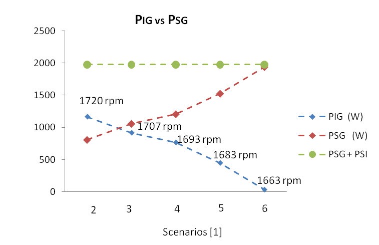Figure 10. PIG vs PSG with DCM_IG field flux variation and V_aDCM kept constant

Figure 11 and Figure 12 shows that the power range supplied from IG, PIG, through the autotransformer method, is greater than PIG of 234 Vdc through the steady source method. Consequently, the power complement from SG is lower than the PSG from 234 Vdc steady source method. Both methods feed the entire resistive load in Figure 10 and Figure 11, and resistive and motor load as shown in Figure 12.

In Figure 13, Figure 14 and Figure 15 shows the comparative results of IG and SG primary machine output power, P_DCMIG vs P_DCMSG. These performances are similar to PIG and PSG performances shown in Figure 10, Figure 11 and Figure 12. The P_DCMIG in Figure 13 elevates because the flux decreases and V_aDCMIG is kept constant [1] The P_DCMIG in Figure 14 and Figure 15 elevates because of the V_aDCMIG increases, which is manually adjusted by the autotransformer shown in Figure 5 and Figure 6.

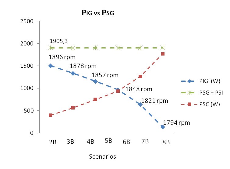Figure 11. PIG vs PSG with V_aDCMIG variation and field flux kept constant (Only resistive load)

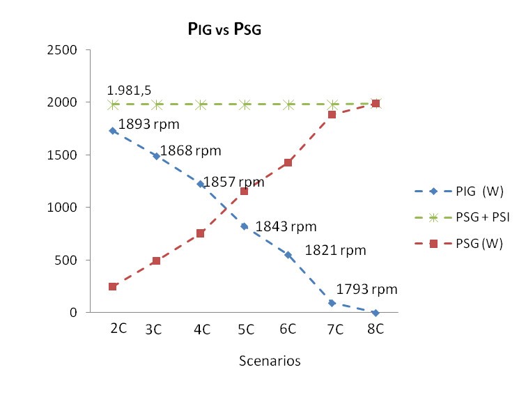Figure 12. PIG vs PSG with V_aDCMIG variation and field flux kept constant (Resistive load plus IM)

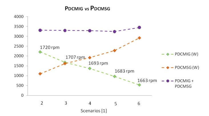Figure 13. P_DCMIG vs P_DCMSG with DCM_IG field flux variation and V_aDCMIG kept constant

The efficiency results shown in Figure 16, Figure 17 and Figure 18 present each subgroup efficiency for each scenario and load conditions. Each subgroup efficiency is resulted from relation between a generator and a DCM as shown in (32) and (33). In summary, the target scenarios are: 2 to 7 (without autotransformer) as in [1], scenarios 2B to 8B (with

autotransformer and just resistive load) and scenarios 2C to 8C (with autotransformer, resistive load and induction motor).

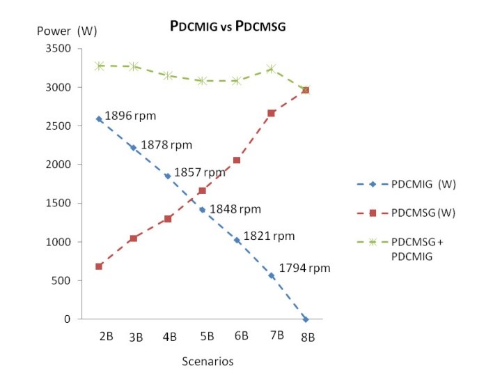Figure 14. P_DCMIG vs P_DCMSG with V_aDCMIG variation and field flux kept constant (Only resistive load)

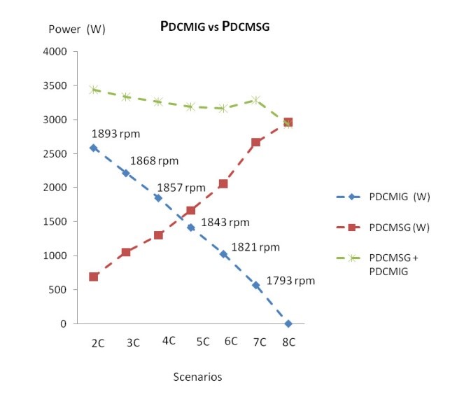Figure 15. P_DCMIG vs P_DCMSG with V_aDCMIG variation and field flux kept constant (Resistive load plus IM)

The IG subgroup efficiencies shown in Figure 17 and Figure 18 are bigger than IG subgroup efficiencies from similar scenarios in Figure 16. Moreover, the elevation of power from IG due to the increase of DCM_IG speed, n_IG, is more representative of actual offshore conditions. The turbines can assume whatever speed required from generators in offshore platforms.

The reduction of losses contributed to increased IG subgroup efficiency as shown in Figure 17 and Figure 18. Fig. 16 shows the machine’s efficiencies when the I_fDCMIG decreases to elevate the speed. The efficiency improves when the V_aDCMIG elevation method is applied as shown in Figure 17 and Figure 18.

The Figure 17 and Figure 18 are higher than the efficiency presented in Figure 16 considering that the Figure 16 indicates a DCM_IG speed range is more restricted as already clarified in [1].

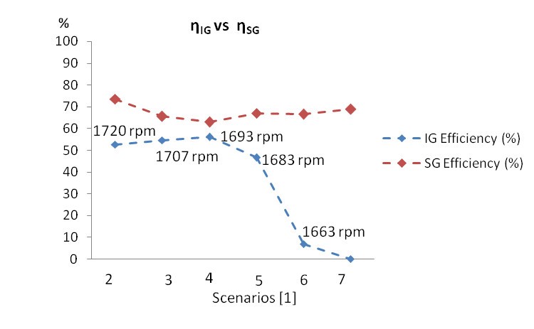Figure 16. η_IG vs η_SG with DCM_IG field flux variation and V_aDCMIG kept constant

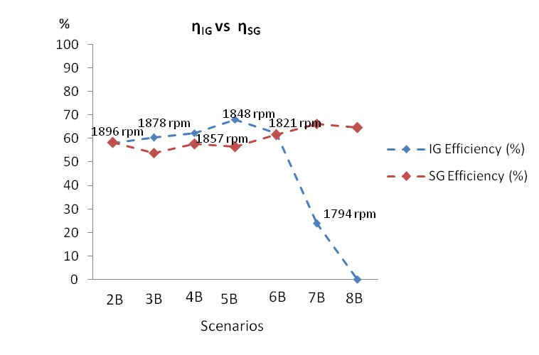Figure 17. η_IG vs η_SG with V_aDCMIG variation and field flux kept constant (Only resistive load)

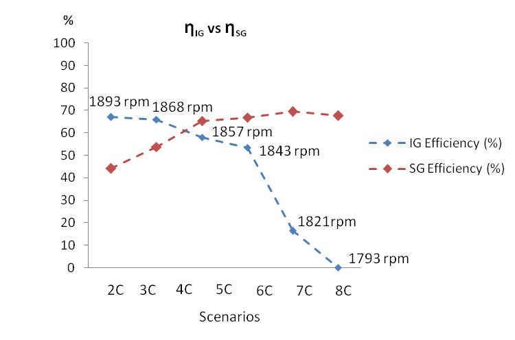Figure 18. η_IG vs η_SG with V_aDCMIG variation and field flux kept constant (Resistive load plus IM)

5. Conclusion

The cited electric system shows voltage and frequency regulation for each scenario transition as demonstrated by results and respective analysis.

As it happened in [1], it was realized the master and slave behaviors to respectively SG and IG. SG controls the system voltage and frequency and IG follows the voltage and frequency defined by SG. The IG establishes the active power supplied to the system and the SG complements the rest of active power and reactive power required. The PIG depends on the IG shaft speed imposed by DCM_IG. The PSG and the system voltage and frequency are controlled by voltage and speed control loops presented in Figure 5 and Figure 6.

It was realized a greater PIG range in the scenarios in Table 7 and in Table 8, than the scenarios from [1] due to V_aDCMIG elevation method. The PSG complemented the PIG manually set to attend the load.

 The V_aDCMIG elevation method resulted in increase of P_DCMIG and PIG and higher IG subgroup efficiency than the I_fDCMIG reduction method[1]. The increase of P_DCMIG and PIG were results of IG speed increase, n_IG, that was obtained by elevation of V_aDCMIG as shown in Figure 11, Figure 12 and Figure 14. The use of V_aDCMIG range instead of Vdc steady source enables to reach the I_aDCMIG limit of 8,0 A and 1893 rpm shaft speed, it is 5,16% higher than synchronous speed. It is higher than Vdc steady source method limit that reached just 4,24% higher than synchronous speed, Figure 16 and [1].

The efficiencies from the V_aDCMIG elevation method were greater than efficiencies from the scheme with Vdc steady source [1], as shown in Figure 17 and Figure 18. V_aDCMIG elevation method does not have the additional current losses of Vdc steady source method. When the field flux ϕ, I_fDCMIG, is decreased, I_aDCMIG is increased by (3) and IG speed, n_IG, is increased by (2). The main losses for the Vdc steady source method are related to higher I_aDCMIG elevation, P(w)=Ra* I_aDCMIG². Then, by the Vdc steady source method, besides I_aDCMIG be elevated due to the rise of PIG, I_aDCMIG is also elevated due to reduction of I_fDCMIG. Higher I_aDCMIG result in higher losses and lower efficiencies.

As shown in power performance graphs related to the V_aDCMIG elevation method, Figure 11, Figure 12, Figure 14 and Figure 15, the PIG and P_DCMIG are more representative of actual operation conditions in offshore platforms.

In continuation of this content, a study of load and generation transients has been done and submitted to publication in COBEP, Brazilian Power Electronic Conference that took place in November, 2017.

In the next stage of this work, it will be studied energy regeneration and ballast load as a additional way to the system regulation.

Conflict of Interest

The authors declare no conflict of interest.

Acknowledgment

The authors would like to thank the UNIFEI and PETROBRAS for the general support along the study.

Appendix 1_ Induction Motor Parameters

The follow calculus were developed on base in [7].

1. No Load and Locked Rotor Tests

The Figure 1 shows the circuit implemented in laboratory to no load test and locked rotor test.

The temperature during the test= 26ºC.

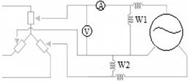Figure 1: No load test and locked rotor test circuit

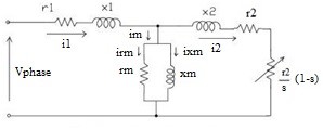Figure 2: Induction Motor Equivalent Circuit

The Figure 2 shows the induction motor IM equivalent circuit.

1.1.  No Load Test

In this section, it will be presented the no load test and locked rotor test to calculus the IM parameters such as impedances, currents, losses and efficiency

The Table 1 presented the no load test measurements.

Table 1: No load Test

Vapply (V)	W1 (W)	W2 (W)	V (V)	A (A)	W1+W2(W)
240	-120.0	+220.0	240.2	1.50	100.0
220	-100.0	+170.0	220.8	1.35	70.0
200	-70.0	+130.0	200.3	1.15	60.0
180	-60.0	+110.0	180.3	1.00	50.0
160	-40.0	+80.0	160.0	0.90	40.0
140	-30.0	+60.0	140.0	0.75	30.0
120	-20.0	+45.0	120.0	0.65	25.0
100	-15.0	+30.0	100.1	0.55	15.0
80	-10.0	+20.0	80.0	0.50	10.0
60	-4.0	+12.5	60.0	0.25	8.5
40	0.0	+5.0	40.0	0.15	5.0
20	0.0	+2.0	20.1	0.05	2.0
0	0.0	0.0	1.99	0.0	0.0

Figure 3 shows the curve of voltage applied and power measured by wattmeter (w1) and (w2). Note that the cross of curve and vertical axe result in estimated attrition and ventilation losses (Pav). In this case Pav is 1 W as demonstrated.

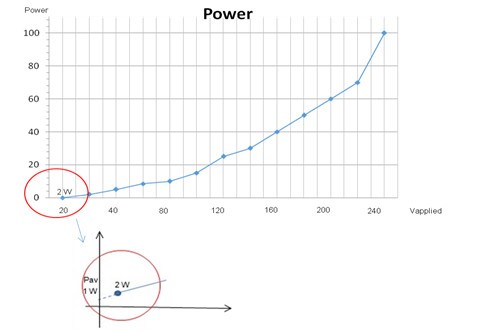Figure 3: Results of no load test: W1+W2 vs Voltage applied

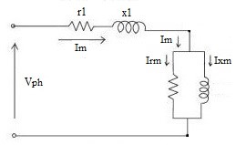Figure 4: Equivalent circuit – No load test

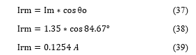
• Magnetization Current

Im = Magnetization Current

Im= 1.35 A as shown in Table 1.

1.2.   Locked Rotor Test

The Table 2 shows the locked rotor test measurements.

Table 2 Locked Rotor Test

W1 (W)	W2 (W)	V  (V)	In   (A)	W1+W2 (W)
20	65	39.34	1.80	85

• Rated Current

In = Rated Current

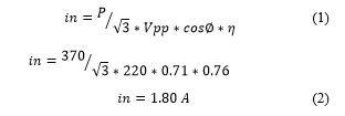The Figure 3 shows the induction motor IM equivalent circuit during locked rotor test

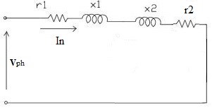Figure 5: Equivalent circuit _ Locked rotor test

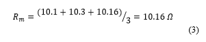
1.3.  Magnetization Branch Parameters

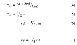
Rm= Motor Average Measured Resistance

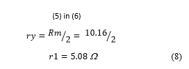
ry=  Phase resistance in star connection

rd=  Phase resistance in delta connection

Table 3: Average Resistance

RAA’	RBB’	RCC’
10.1	10.3	10.16

• r1 Calculus

Follow the calculus memory of stator winding resistor r1.

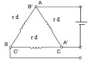Figure 6: IM winding connection

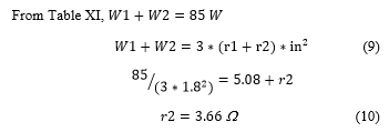
• r2 Calculus

From Table XI,

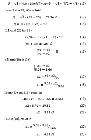
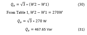
• Reactive Power

2. Power and Losses Calculus

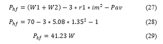
The  was defined in Figure 3 and consist in 1 W and Pnl (no load losses) is no load test for 220 V, it resulted in 70 W (W1 +W2).

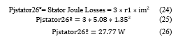
• Stator Joules Losses

• Phf_ histerese and foucault losses

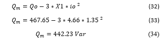
1.4.  No Load Reactive Power

1.5.  Magnetization Branch

• No load Reactive Power in Magnetization Branch

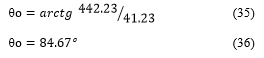
• Magnetization Branch Power Factor Angle

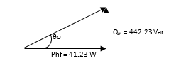Figure 7: Magnetization branch power factor

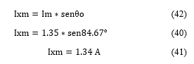
• Magnetization Branch Currents

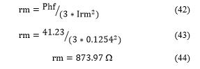
• Magnetization Branch Resistance

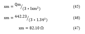
• Magnetization Branch Reactance

3. Parameters of Induction Motor

Figure 8 shows all IM parameters calculated as resistors, reactance and currents as data obtained during experiment, without temperature correction because the motor operated no load.

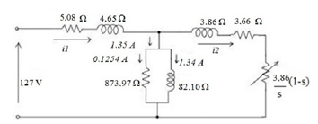Figure 8: Parameters of Induction Motor _IM

4. Induction Motor Efficiency

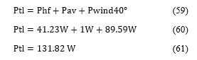
It will be calculated the temperature correction factor, corrected resistences to 40ºC, corrected winding losses, Pwind40ºC, and total losses, Ptl, before induction motor efficiency calculus.

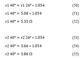
1.6.  Temperature Correction Factor and Resistence Correction

• Temperature Correction Factor Kt 40ºC

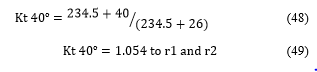• Resistence Correction

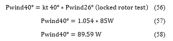
1.7.  Corrected Winding Losses and Total Losses

• Winding Losses

The winding losses, Pwind, measured in locked rotor test, Table 2, need to be corrected to 40ºC. Follow the corrected winding losses.

• Total Losses

The total losses, Ptl, calculus:

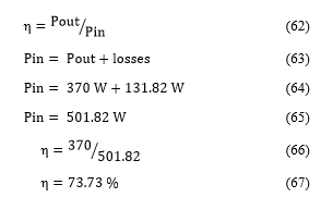
1.8.  Rated Motor Efficiency Estimate

Pout = Motor output power (Motor dataplate_Table 6)

Pin=Motor Input power

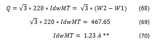
5. Induction Motor Currents

Follow the calculus of IM reactive and active currents (IdwMT and IwMT). This values are shown in Table 8 for all scenarios tested.

• Reactive Current

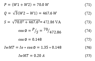
** The difference between IdwMT and Ixm is perfectly acceptable. The difference close to 0,1 A between expected and found values is due to small measurements errors and instruments precision and accuracy errors. It does not impact the presented modeling. Therefore, the results and modeling continue valid.

• Active Current

In Figure 9 are shown resistor banks current and no load IM current.

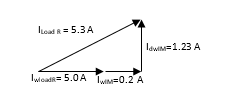Figure 9: Resistors bank and IM currents in scenarios C

1.  V. Z. Silva, A. J. J. Rezek, and R. L. Corrêa, “Analysis of synchronous and induction generators in parallel operation mode in an isolated electric system”, Brazil, 2017, https://doi.org/ 10.1109/PEDG.2017.7972459
2. S.P. Singh., B. Singh, M.P. Jain, “Comparative study on the performance of a commercially designed induction generator with induction motors operating as self-excited induction generators”, IEE Proc. C, vol. 140, no.5, pp: 374 – 380, 1993, https://doi.org/ 10.1049/ip-c.1993.0055
3. M. H. Haque, “Self-excited single-phase and three-phase induction generators in remote areas”, IEEE conference, pages 38-42, 2008, https://doi.org/ 10.1109/ICECE.2008.4769169
4. E. Touti, R. Pusca, J. F. Brudny, A. Châari, “Asynchronous generator model for autonomous operating mode”, IEEE conference, pages 1-3, 2013, https://doi.org/ 10.1109/ECAI.2013.6636208
5. D. M. Macedo, “The use of pumps operating as turbines and induction generators in electric power generation” (in Portuguese), Master in Science Dissertation, Federal University of Itajubá(UNIFEI), Itajubá, 2004.
6. J. M. Chapallaz, P. Eichenberger, and G. Fischer, Manual on Pumps used as Turbines. MHPG Series, v. 11, Friedr. Vieweg&SohnVerlagsgesellschaftmb, Germany, 1992.
7. J. R. Cogo, J.C. Oliveira, and J. P. G. Abreu, “Tests in induction machines”, editor EFEI, Itajubá-MG, Brazil, 1983.
8. A. P. Rizzi, ” Electrical Measurements: power, energy, power factor, demand”, in Portuguese, Livros Técnicos e Científicos Editora S.A., Rio de Janeiro-RJ, 1980.

(Click to view)

(Click to view)