1. Introduction

Actuator faults may cause undesired system behaviour and sometimes lead to instability, hence it is necessary to develop Fault Tolerant Control (FTC) methods against actuator faults of uncertain nonlinear systems. In the past decades some FTC design methods have been proposed for several classes of nonlinear systems with actuator faults [1-3]. It consists in computing control laws by taking into account the faults affecting the system in order to maintain acceptable performances and to preserve stability of the system in the faulty situations [4]. From the point of view of FTC strategies, the literature considers two main groups of techniques: passive and active ones. In passive FTC, the faults are treated as uncertainties. Therefore, the control is designed to be robust only to the specified faults [4]. Active FTC techniques consist in adapting the control law using the information given by the Fault Detection and Isolation (FDI) block [5]. The informations issued from the FDI block are used by the FTC module to reconfigure the control law in order to compensate the fault and to ensure an acceptable system performances. The study of this problem was extended to switched systems in [6-8]. In [7], a switched discrete-time system with state delay has been considered. The design method is based on the construction of a filter and a fault estimation approach. In [8], an adaptive fuzzy tracking control method for a class of switched nonlinear systems with arbitrary switchings and with actuator faults has been proposed. The proposed control scheme guarantee the stability of the whole switched control system based on the common Lyapunov function stability theory and attenuate the effect of the actuator faults on the control performance by designing a new fuzzy controller to accommodate uncertain actuator faults. In [9], an observer has been built to detect the fault when it occurs. The problem of FTC for switchied linear systems is addressed by using a nominal control law designed in the absence of any fault, associated with fault detection, localization and reconfiguration techniques to maintain the stability of the system under an arbitrary switching signal in the presence of sensor faults. A state trajectory tracking has been proposed in [4] for actuator faults and observer bank based on controllers with switching mechanism for sensor faults has been also presented in [10]. A nonlinear observer based controller, adopting the so-

called parallel distributed compensation structure, has been designed to choose an adequate state estimate to compensate the effects of the faults on the system in [11]. Switched systems are dynamical systems consisting of a collection of continuous-time subsystems. Switched systems have attracted more attention due to their significance in the modelling of many engineering applications, such as chemical processes, robot manipulators and power systems. Stability analysis and synthesis of switched systems have been made using Lyapunov function to ensure stability of the switched systems such in [12].

In this paper, in order to acheive the FTC for a switched discrete-time systems, a set of PID-type Fuzzy Logic Controller (FLC) is implemented to minimize the error between the desired flat trajectory and the estimated state and to maintain the stability of the system in the presence of actuator faults. The estimated state is provided from an Unknown Input Observer (UIO). Based on residual analysis, a switching strategy using stateflow is then designed. The global stability for the switched systems is studied by Lyapunov theory and expressed as a Linear Matrix Inequalities (LMIs).

The paper is organized as follows. In Section 2, the FTC problem statement is formulated. In Section 3, the fault detection method using UIO is introduced. In Section 4, the PID-type FLC is described. Section 5 deals with the flatness property. The proposed approach is applied to an ETV in Section 6. Finally, the conclusion is drawn in Section 7.

2. FTC problem statement

Consider the discrete time switched system, which can be formulated such that

x(k +1) = A_jx(k)+B_ju(k)+E_jd(k)+B_jf_a(k)             (1) y(k) = C_jx(k)

x(k) ∈ Rⁿ is the state vector, u(k) ∈ R^p the control input, _y(_k) ∈ R^o the measured output, _d(_k) ∈ R^p the unknown disturbance input and _fa(_k) ∈ R^p the ac-

tuator faults. A_j ∈ R^n×n, B_j ∈ R^n×p, C_j ∈ R^o×n and _Ej ∈ R^n×p are the known constant matrices for j ∈ _ψ = {1_,2_,…,m} and _m the number of models,

m > 1.

In this paper, a FTC structure based on PID-type FLC, given by Figure 1, is proposed to maintain the trajectory tracking and to preserve stability of ETV in the presence of both input disturbance _d(_k) and actuator faults _fa(_k).

According to this structure, the FTC approach needs to detect actuator faults firstly and then to design the j^th control law, denoted _uj(_k) given by (2), in order to minimize the error between the desired flat trajectory, generated using the flatness property and the estimated state, provided from the _j^th UIO.

                                 u_j(k) = −K_c,jxˆ_j(k)+y_j^d(k)                            (2)

K_c,j is the _j^th gain control law.

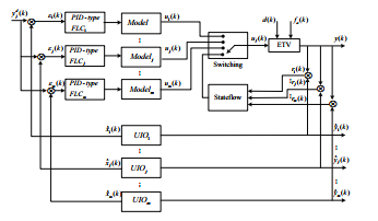Figure 1: Proposed structure of FTC approach

In this case, LMI-based UIOs for the switched system (1) are designed using Lyapunov function for arbitary switching signal. Then, residuals _rj(_k) are determined by the UIOs and employed to achieve actuator faults detection.

3. Unknown input observers design and stability analysis

In this section, let us consider _fa(_k) = 0, then the model (1) becomes x(k +1) = A_jx(k)+B_ju(k)+E_jd(k) (3)

y(k) = C_jx(k)

j _{∈ ψ} denotes the _j^th model. The structure of full rank UIOs can be formulated by z(k +1) = F_j(k)+T_jB_ju(k)+K_jy(k) (4) xˆ(k) = z(k)+H_jy(k)

where ˆ_x(_k) is the estimated state vector _x(_k), _z(_k) is the state vector of full rank UIOs. _Fj, _Tj, _Kj and _Hj are unknown matrices which need to be designed. Lemma: [13] Equation (4) is UIO of the switched system (3), if and only if the following conditions are satisfied

• rank(C_jE_j) = rank(E_j)
• (C_jA_j1) is observable with

Aj1 = Aj −Ejh(CjEj)T CjEji−1(CjEj)T CjAj (5) According to the above, the formulation of UIOs is constructed for each subsystem. In the next part, the multiple Lyapunov function will be used to realize the design of parameters for UIOs of switched system. Theorem: [14] In the condition of arbitrary switching signal, for the system (3), if

                                         (H_jC_j −I)E_j = 0                                     (6)

T_j = (I −H_jC_j)

Fj = (Aj −HjCjAj −Kj1Cj)

Kj2 = FjHj hold, and there exist symmetric matrices _Pj > 0, ∀_j ∈ ψ such that

                            −TPPjj            P−jPFjj6 0, ∀j ∈ ψ                       (7)

Fj then the parameters of UIOs can be designed. Proof: Define the state estimation error as _e(_k) = x(_k)_−xˆ(_k), the dynamic equation can be derived as

e(k +1) = (A_j −H_jC_jA_j −K_j1C_j)e(k)

−Fj −(Aj −HjCjAj −Kj1Cj)z(k) −Kj2 −(Aj −HjCjAj −Kj1Cj)Hjy(k) −T_j −(I −H_jC_j)B_ju(k)−(H_jC_j −I)E_jd(k)

(8)

with

                                           Kj = Kj1 +Kj2                                                         (9)

In order to make the error decoupled from known control input _u(_k), measured output _y(_k) and unknown input _d(_k), we should let

(HjCj −I)Ej = 0 Tj −(I −HjCj) = 0 Fj −(Aj −HjCjAj −Kj1Cj) = 0 Kj2 −(Aj −HjCjAj −Kj1Cj)Hj = 0 It can be concluded that	(10)
Hj = Ej (CjEj)T CjEji−1(CjEj)T h	(11)
Aj1 = Aj −Ej (CjEj)T CjEji−1(CjEj)T CjAj h	(12)
Fj = Aj −HjCjAj −Kj1Cj = Aj1 −Kj1Cj and the error dynamics is given by	(13)
e(k +1) = Fje(k)	(14)

Equation (4) is UIOs of the switched system (3) if the estimation error tends asymptotically to zero despite the presence of an unknown input _d(_k) , 0. Consider the following Lyapunov function

                                   V_j(e(k)) = e(k)^T P_je(k)                           (15)

For P_j = P_j^T > 0, then, V_j(e(k)) > 0 holds, the _∆V

given by (16) is negative

V_i(e(k +1))−V_j(e(k))

                       = e(k)^T F_j^T P_iF_je(k)−e(k)^T P_je(k)                         (16)

P_iF_j −P_j)e(k);(i ∈ ψ,j ∈ ψ,i , j)

if the following inequalities are satisfied

                                         F_j^T P_iF_j −P_j 6 0                                  (17)

Thus, the error system (14) is stable asymptotically. According to Schur complement lemma, the inequalities (17) can be rewritten as

                                     −TPPii         P−iPFjj6 0                            (18)

Fj

By substituting F_j = A_j1 − K_j1C_j, the above matrix

inequalities become

−Pi (Aj1 −Kj1Cj)T Pi and	Pi(Aj1 −Kj1Cj) −Pj	< 0	(19)
−Pi (PiAj1 −WijCj)T	(PiAj1 −WijCj) −Pj	< 0	(20)

for Wij = PiKj1.

Since K_j1 = P_j⁻¹W_ij, we can obtain the value of K_j1 then F_j, K_j2 and K_j = K_j1 + K_j2 from P_j and W_ij solutions of LMIs.

The aim of fault detection is to generate a residual signal _rj(_k), given by (21), which is sensitive to _fa(_k) in the presence of actuator faults which is the purpose of

[15].

                                    r_j(k) = y(k)−C_jxˆ_j(k)                             (21)

4. PID-type fuzzy logic controller design

In this study, the FTC approach is based on PID-type FLC. To adjust the input and the output scaling factors of this controller, Genetic Algorithm (GA) optimization technique has been proposed in order to improve the performance of the controller.

4.1         PID-type fuzzy logic controller description

We consider a PID-type FLC structure as shown in

Figure 2, [16], where K_e ∈ R⁺ and K_d ∈ R⁺ are the input scaling factors, _α ∈ R⁺ and _β ∈ R⁺ the output scaling factors.

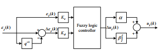Figure 2: The PID-type FLC

The FLC inputs variables, the error _εj(_k) between the desired flat trajectory _yj^d(_k) and the estimated state xˆ(_k), and error variation _∆εj(_k) are given by the equations (22) and (23) where _Te is the sampling period. ε_j(k) = −K_c,jxˆ(k)+y_j^d(k) (22)

                  ∆εj(k) = εj(k)−εj(k −1)           (23)

T_e

The output variable _∆uj(_k) of a such controller is the variation of the control law signal _uj(_k) which can be defined as (24).

                 ∆uj(k) = uj(k)−uj(k −1)          (24)

T_e

The output of the PID-type FLC is given by (25), [17]

Z

u_j(k) = α∆u_j(k)+β ∆u_j(k) dt

= α(A+QK_eu_j(k)+DK_d∆u_j(k))

+β^Z (A+QK_eu_j(k)+DK_d∆u_j(k)) dk

= αA+βAk +(αK_eQ+βK_dD)u_j(k)

+βK_eQ^Z u_j(k) dk +αK_dD∆u_j(k)

(25)

where the terms _Q and _D are given by (26) and (27),

[10].

_Q = ∆u(i+1)^j −∆uij (26) εi+1 −εi

∆^u_i(j+1) −∆uij

                                  D =                           (27)

∆ε_j+1 −∆ε_j

The fuzzy controllers with product₋sum inference method, centroid defuzzification method and triangular uniformly distributed membership functions for the inputs and a crisp output proposed in [18], are used, in our study.

The linguistic levels, assigned to the variables _εj(_k),

∆_εj(k) and _∆uj(_k), are given in Table 1 as follows: NL: Negative Large; _N: Negative; _ZR: Zero; _P: Positive; _PL: Positive Large.

εj(k) / ∆εj(k)	N	ZR	P
N	NL	N	ZR
ZR	N	ZR	P
P	ZR	P	PL

Table 1: Fuzzy rules-base

4.2         Optimization of scaling factors using genetic algorithm

To adjust the input and the output scaling factors (_Ke, K_d) and (_α, _β), GA is used in order to obtain their optimal values.

At first, an initial chromosome population is randomly generated. The chromosomes are candidate solutions to the problem. Then, the fitness values of all chromosomes are evaluated by calculating an objective function. So, based on the fitness of each individual, a group of the best chromosomes is selected through the selection process. The genetic operators, crossover and mutation, are applied to this ’surviving’ population in order to improve the next generation solutions. Crossover is a recombination operator that combines subparts of two parent chromosomes to produce offspring. This operator extracts common features from different chromosomes in order to achieve even better solutions. Mutation is an operator that introduces variations into the chromosome. The modifications can consist of changing one or more values of a chromosome. Through the mutation operator the search space is explored by looking for better points. The process continues until the population converges to the stop criterion.

The most crucial step in applying GA is to choose the objective function that is used to evaluate the fitness of each chromosome. In this paper, the method of tuning PID-type FLC parameters using GA is based on minimizing the Integral of the Squared Error (ISE) used in

[18].

5. Flatness and trajectory planning

The flatness approach is used in a discrete-time framework for system (1). Let the studied dynamic linear discrete system described by (28)

D_j(q)y_j(k) = N_j(q)v_j(k) (28) q is the forward operator, _vj(_k) and _yj(_k) are, respectively, the input and the output signals and _Dj(_q) and N_j(_q) the polynomials defined by

                  Dj(q) = qn +aj,n−1qn−1 +…+aj,1q +aj,0                            (29)

Nj(q) = bj,n−1qn−1 +…+bj,1q +bj,0 (30) where the parameters _aj,l and _bj,l are constants, _l =

{0,1,…,n−1}.

The system is considered as linear and controllable, consequently it is flat, [16].

The flat output _zj(_k), on which depend the output y_j(_k) and the control _vj(_k), can be seen as being the partial state of a linear system, [19]

v_j(k) = D_j(q)z_j(k)        (31) y_j(k) = N_j(q)z_j(k)             (32)

The open loop control law can be determined by the following relations, [18]

v_j^d(k) = f(z_j^d(k),…,z_j^d(r+1)(k)) (33) y_j^d(k) = g(z_j^d(k),…,z_j^d(r)(k)) (34) f and _g are vectorial functions and _zj^d(_k) is the desired trajectory that must be differentiable at the (_r + 1) order.

In order to plan the desired flat trajectory _zj^d(_k), the polynomial interpolation technique is used.

Let       consider      the      state      vector:            _Zj^d(_k)        =

(z_j^d(k) z_j^d(1)(k) … z_j^d(r+1)(k))^T containing the desired flat output and its successive derivatives, [18]. The expression of _Zj^d(_k) can be given as following where _k0 and _kf are two moments known in advance.

Zjd(k) = Mj,1(k −k0)cj,1(k0)+Mj,2(k −k0)cj,2(k0,kf)

(35)

such that

                                      1       k       ···     (knn−−1)!1 

Mj,1 = …   0

… ···

… 0

(n−2)!  …  1

(36)

                                      0       1       ···         k(n−2)

                               n                    n+1                                          2n−1

 k n!  kn−1 = (n−1)! Mj,2                         …    k	k (n+1)! kn n! … ···	··· ··· … kn−1 (n−1)!	k                      (2n−1)! k(n−2)  (n−2)!  …                 kn  n!	(37)
	cj,1 = Zjd(k0)			(38)

cj,2 = Mj,−21(kf −k0)(Zjd(kf)−Mj,1(kf −k0)Zjd(k0))

(39) After planning a desired flat trajectory in discrete-time framework, the real output _yj(_k), to be controlled, follows the desired trajectory _yj^d(_k) such that (40), [18].

                                     y_j^d(k) = N_j(q)z_j^d(k)                              (40)

6. Application of an electronic throttle valve

6.1        Electronic throttle valve modeling

The proposed approach is applied here for the case of the electronic throttle valve, Figure 3, [15].

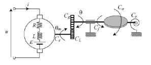Figure 3: Electronic throttle system

The electrical part of this system is modeled by (41), [20,21].

                           u(t) = Ri(t)+L ^d i(t)+k_vω_m(t)                   (41)

dt

L is the inductance, _R the resistance, _u(_t) and _i(_t) the voltage and the armature current respectively, _kv a constant electromotive force and _ωm(_t) the motor rotational speed.

The mechanical part of the throttle is modeled by a gear reducer, characterized by its reduction ratio _γ such as (42)

                                            γ = ^Cg                                                        (42)

C_L

C_L is the load torque and _Cg the gear torque.

The mechanical part is modeled according to (43) and (44), such that, [20,21]

d J  ωm(t) = Ce −Cf −Cr −Ca dt	(43)
d θ(t) = (180/π/γ)ωm(t)	(44)

dt

θ(_t) is the throttle plate angle, _Ce the electrical torque, C_f the torque caused by mechanical friction, _Cr the spring torque, _Ca the torque generated by the airflow and _J the overall moment of inertia. The electrical torque is defined by

C_e = k_ei(t)       (45) where _ke is a constant.

The electronic throttle valve involves two complex nonlinearities due to _Cr and _Cf, given by their static char-

acteristics, [15]

• a dead zone in which the control voltage signal has no effect on the nominal position of the valve

plate,

• two hysteresis combined with a saturation, due to the valve plate movement, limited by the maximum and the minimum angles. The static characteristic of the nonlinear spring torque C_r is defined by

C_r = ^kr (θ −θ₀)+Dsgn(θ −θ₀)      (46) γ

for θ_min 6 θ 6 θ_max, k_r is the spring constant, D a constant, _θ0 the default position and sgn(_.) the following signum function

sgn(θ −θ0) =  1, 1if,θelse> θ0     (47) −

The friction torque function _Cf of the angular velocity of the throttle plate can be expressed as

                                     C_f = f_vω +f_c sgn(ω)                              (48)

where _fv and _fc are two constants. By substituting in equation (43), the expressions _Ce, C_f and _Cr and by neglecting the torque generated by the airflow _Ca, the two nonlinearities sgn(_θ −_θ0) and sgn(_ω) and the two constants ^k_γ^r_θ0 and _fv, the studied system is linear then it can be modelized by the following transfer function _H(_s) (49), [21]

^H(^s) = JLs³ +JRs(180² +(/π/γ_kek_v)+k_eLks)s+Rk_s (49) with _ks = (180_/π/γ²)_kr and _s the Laplace operator; the identified parameters of this system are given in Table 2 at 25^◦_C, [20].

Parameters	Values	Units
R	2.8	Ω
L	0.0011	H
ke	0.0183	N.m/A
kv	0.0183	v/rad/s
J	4×10−6	kg.m2
γ	16.95	–

Table 2: Model’s parameters

Recent work has shown that the ETV can be modeled by two linear models identified from the default position of the throttle plate for two values of the parameter _ks and for the sampling period _Te = 0_.002_s,

[21]

• a model representing the position of the plate above the position by default for: _ks = 1_.877 _× 10⁻⁴_m², then the corresponding discrete-time transfer function _H1(_q⁻¹) given by (50),

H1(q−1)= 0.1007480−1.948q−q1−+01 +0.01334.954qq−−22−+00..0061520007376q−q3−3

(50)

• a model representing the position of the plate below the position by default for: _ks = 1_.384 _× 10⁻³_m², then the corresponding discrete-time transfer function _H2(_q⁻¹) given by (51),

                                           −1                                 −2                                      −3

H₂(q−1)= 0.1007479−1.946q q₋+0₁ +0.01333.954qq₋₂ −+00..0061520007376q₋q₃

(51)

6.2        Simulation results

In order to test the proposed fault tolerant control approach, tow models of an ETV in actuator fault and an unknown disturbance case are given as state space formulation as x(k +1) = A_jx(k)+B_ju(k)+E_jd(k)+B_jf_a(k) (52)

y(k) = C_jx(k)

where the parameter matrices and vectors of each model are given as

1.948       – 0.954     0.006152 A1 =  1                  0                  0         0              1                  0	(53)
1.946       – 0.954     0.006152 A2 =  1                  0                  0         0              1                  0	(54)
B1 = B2 = 1        0      0T	(55)
C1 = 0.007480         0.01334     0.0007376	(56)
C2 = 0.007479         0.01333     0.0007376	(57)
E1 = E2 = 1        1     1T	(58)

The studied system fulfills the conditions of Lemma 1.

rank((CC₂¹EE₂¹) = rank(E¹) = 1     (59) rank                ) = _rank(_E2) = 1

then (C₁A₁₁) and (C₂A₂₁) are both observable. By applying Theorem, the system is stable asymptotically for any switching signal for symmetric matrice _P definite positive given by (60).

                              ^ 0.1429          – 0.0857     0.1903^

P = e – 010_ – 0.0857     0.5085   0.0494_ (60) 0.1903           0.0494   0.4251

Then, the rest parameters of UIOs are calculated as below

                      ^ – 0.0266        0.8566         – 1.5415^

             F₁ = _ – 0.0078          0.1954         – 0.3515_              (61)

                          0.0165        – 0.4329       0.7788

 – 0.0233   0.8717   – 1.5349 F2 =  – 0.0071   0.1998   – 0.3515 0.0148        – 0.4384       0.7715	(62)
 0.9657 – 0.6187 – 0.3470 T1 =  – 0.0343 0.3813 – 0.3470 – 0.0343       – 0.6187       0.6530	(63)
 0.9672 – 0.6196 – 0.3476 T2 =  – 0.0328 0.3804 – 0.3476 – 0.0328       – 0.6196       0.6524	(64)
 0.0002                     0.0182  K1 =  0.0031 ,K2 =  0.0208  – 0.0056                       – 0.0389	(65)
46.3945                46.4707 H1 = 46.3945,H2 = 46.4707 46.3945                     46.4707	(66)

In this study, the method of tuning PID-type FLC parameters using GA is based on minimizing the ISE. If y_j^d(_k) is the desired flat trajectory and ˆ_xj(_k) the estimated state, then we have

εj(k) = −Kc,jxˆj(k)+yjd(k) For the ISE defined by	(67)
t Z ISE =         ε2j(k)dt	(68)

0

In this paper, the considered fitness function is taken as inverse of this error, i.e. the following performance index

                                  fitness value =        1                            (69)

ISE Then, the obtained optimum values of the input/output scaling factors (_Ke,K_d,α,β), using genetic algorithm are given as follows: _Ke = 0.2006, _Kd = 0.8071, _α = 0.1146 and _β = 0.2063. The desired discrete time flat trajectory _zj^d(_k), with j = _{1_,2_} can be computed according to the following polynomial form

zjd(k) = PolyBBcstcstj1_j,j(1)2¹(,k,)ifif 0, kif16k<0kk<66kkk6⁰2 k1                (70)

(1)

Poly2B,jcst_j((1)k1),, ifif k > kk2 < k3 6 k3

where _cst1 and _cst2 are constant parameters, _k0 = 3_s, k₁ = 6_s, _k2 = 10_s and _k3 = 15_s are the instants of transitions, _Bj(1) is the static gain between the flat output z_j(_k) and the output signal _yj(_k) for each model and Poly_1,j(k) and Poly_2,j(k) are polynomials calculated using the technique of polynomial interpolation.

The desired trajectories _y1^d(_k) and _y2^d(_k) are then given in Figure 4.

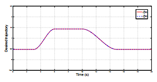Figure 4: Desired trajectories y₁^d(k) and y₂^d(k)

Let us consider the fault vector
fa2 (             fT              fa k) =     aT1((kk)) such as fa2 = 0 and fa1 defined as follows	(71)
, k ∈ [0,10] fa1(k) = −0.1sin(0.314k), k ∈ ]10,13]	(72)

                                           0,                k ∈ ]13,20]

The simulation results illustrated in Figure 5 and Figure 6, show some oscillations for the outputs signals and for the tracking error due to the unknown input. We remark that the system’s responses with and without FTC track desired trajectories with disturbances rejection.

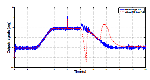Figure 5: System outputs in actuator fault case with and without PID-type FLC

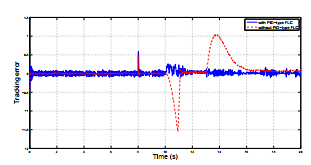Figure 6: Tracking error in actuator fault case with and without PID-type FLC

At the time of actutor faults occurrence _k = 10_s, the system’s behavior was changed. The system without FTC becomes unstable, whereas for the same reference input and by using the FTC, the system remains stable and the tracking error have a small deviation from zero which shows the effectiveness of the proposed FTC approach.

Figure 7, Figure 8 and Figure 9 show the residual values generated using UIOs and the switched signal. The switching between the two models is acheived based on residual values comparision.

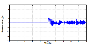Figure 7: Residual value r₁(k) in actuator fault case with PIDtype FLC

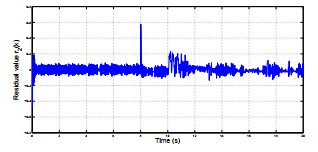Figure 8: Residual value r₂(k) in actuator fault case with PIDtype FLC

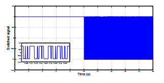Figure 9: Switched signal in actuator fault case with PID-typeFLC

7. Conclusion

In this paper, a new fault tolerant control law based on PID-type FLC is designed for the nonlinear complex system ETV, modelized by a multimodel structure. The approach is based on the use of a reference model generated using the flatness property. The proposed control law is, then, designed to minimize the error between the desired flat trajectory and the estimated state, generated using UIOs, even in the presence of actuator faults based on minimizing the ISE.

1. Y. Huo, Y.M. Li and S.C. Tong, Fuzzy adaptive faulttolerant output feedback control of multi-input and multioutput non-linear systems in strict-feedback form, IET Control Theory and Applications, 6, 2704–2715, 2012.
2. K. Shen, B. Jiang and V. Cocquempot, Fuzzy logic system-based adaptive fault-tolerant control for nearspace vehicle attitude dynamics with actuator faults, IEEE Transactions on Fuzzy Systems, 21, 289–300, 2013.
3. C. Tong, B.Y. Huo and Y.M. Li, Observer-based adaptive decentralized fuzzy fault-tolerant control of nonlinear large-scale systems with actuator failures, IEEE Transactions on Fuzzy Systems, 2,1–15, 2014.
4. Ichalal, B. Marx, J. Ragot and D. Maquin, Fault tolerant control for Takagi-Sugeno systems with unmeasurable premise variables by trajectory tracking, IEEE International Symposium on Industrial Electronics (ISIE), Bari, 2010.
5. Blanke, M. Kinnaert, J. Lunze and M. Staroswiecki, Diagnosis and Fault-Tolerant Control, Springer-Verlag Berlin Heidelberg, 2006.
6. Nouailletas, D. Koeing and E. Mendes, LMI design of a switched observer with model uncertainty: Application to a hysteresis system, Proc. of the 46th IEEE CDC, New Orleans, 6298–6303, 2007.
7. Wang, W. Wang and P. Shi, Robust fault detection for switched systems with state delays, IEEE Trans. On Systems and Cybernetics-B, 39, 800–805, 2009.
8. Yingxue, T. Shaocheng and L. Yongming, Adaptive fuzzy backstepping control for a class of switched nonlinear systems with actuator faults, International Journal of Systems Science, 47, 3581–3590, 2015.
9. Benzaouia, M. Ouladsine, A. Naamane and B. Ananou, Fault detection for uncertain delayed switching discretetime systems, International Journal of Innovative Computing, Information and Control, 8, 1–11, 2012.
10. Oudghiri, M. Chadli and A. El Hajjaji, Robust observer-based fault tolerant control for vehicle lateral dynamics, International Journal of Vehicle Design, 48, 173– 189, 2008.
11. Ichalal, B. Marx, D. Maquin and J. Ragot, Nonlinear observer based sensor fault tolerant control for nonlinear systems, 8th IFAC Symposium on Fault Detection, Supervision and Safety of Technical Processes, Mexico, 2012.
12. Benrejeb, Stability Study of Two Level Hierarchical Nonlinear Systems, 12th IFAC Symposium on Large Scale Systems: Theory and Applications, 43 (8), 30–41 Villeneuve d’Ascq, 2010.
13. Chen, R.J. Patton and H.Y. Zhang, Design of unknown input observers and robust fault detection filters, International Journal of Control, 63, 85–105, 1996.
14. Jiawei, S. Yi and Z. Miao, Fault Detection for Linear Switched Systems Using Unknown Input Observers, Proceedings of the 33rd Chinese Control Conference, Nanjing, 2014.
15. Gritli, H. Gharsallaoui and M. Benrejeb, Fault Detection Based on Unknown Input Observers for Switched Discrete-Time Systems, Int. Conf. on Advanced Systems and Electrical Technologies IC-ASET, Hammamet, 2017.
16. Bouall`egue, M. Ayadi, J. Hagg´ege and M. Benrejeb, A PID type fuzzy controller design with flatness-based planning trajectory for a DC drive, IEEE International Symposium on Industrial Electronics, Cambridge, 1197–1202, 2008.
17. Guzelkaya, I. Eksin and E. Yesil, Self-tuning of PIDtype fuzzy logic controller coefficients via relative rate observer,Engineering Applications of Artificial Intelligence, 16, 227–236, 2003.
18. Gritli, H. Gharsallaoui and M. Benrejeb, PID-type Fuzzy Scaling Factors Tuning Using Genetic Algorithm and Simulink Design Optimization for Electronic Throttle Valve, International Conference on Control, Decision and Information Technologies CoDIT, Malta, 2016.
19. Fliess, J. L´evine, P. Martin and P. Rouchon, On differentially flat non linear systems, In Proc. IFACSymposium NOLCOS, pp. 408-413, Bordeaux, 1992.
20. Lebbal, H. Chafouk, G. Hoblos and D. Lefebvre, Modelling and Identification of Non-Linear Systems by a Multimodel Approach: Application to a Throttle Valve, International Journal Information and Systems Science, 3, 67–87, 2007.
21. Yang, Model-based analysis and tuning of electronic throttle controllers, Visteon Corporation, SAE 2004 World Congress & Exhibition, 63–67, 2004.

(Click to view)

(Click to view)