1. Introduction

A Synchronous circuits entail several benefits. Firstly performance advantages, e.g. faster system perfomance, no clock synchronization, fewer power consumption and fewer electromagnetic emission. Secondly asynchronous circuits also have safety advantages, e.q. no clock skew. Asynchronous circuits can also lead to simplicity, by connecting different parts modularly [1, 2]. On the other hand asynchronous circuits provide risks, such as faults like hazards, glitches and so on [3]. Therefore it is very important to design asynchronous circuits correctly, especially in safety critical applications such as in automotive, where human lives are at stake. To prevent faults like hazards, a mealyto-moore transformation will be presented, which creates a function stable asynchronous machine. The Mealy machine with the state transfer function δ and the output function λ, see figure 1 be given. Each Mealy machine can be transformed into an equivalent Moore machine [3] for example by increasing the arity of δ by |x| and coding it with x, z0 =(z,x) with δ0(z0,x) 7→ (δ(z,x),x), and the output function is only dependent on the new state variable z0 with µ : (z0) 7→ µ(z0).
By comparing the two machines the pros and cons can be shown. Therefore the idea of transforming the machines into each other to profit from the benefits of both is obvious. Mealy machines have the advantage of requiring less states since one state can produce a number of different outputs in combination with the input. A Moore machine’s state on the other hand only produces one output. A Mealy machine is also faster by reacting directly to the input. This feature however is not always wanted, since it can lead to undesired outputs (e.g. hazards, glitches) when the input is variable. A Moore machine is more stable in this regard, since it only indirectly reacts to input changes. The output only changes when transferring into the next state. Transforming a Mealy machine into a Moore machine is therefore useful in case a direct dependence on the input is to be avoided [2]. In the paper the transformation of a Mealy machine into a Moore machine is presented. The machine will be designed under the use of dual-rail logic and the RS-buffer, and will stabilize itself. Firstly the transformation is made by breaking the feedback up and nesting it in the RS-buffer, secondly by encoding the inputs as states, so that the output function is only dependent on pseudo states. With the method presented in this article, function stable sequential circuit parts can be seen as combinational logic and moved over other blocks at will. With this method, individual machines can be strung together to realize complex circuits for safety relevant applications.

2. Theory

This paper describes the underlying theory of the transformation and provides an illustrative example.
Figure 1 shows a fully asynchronous Mealy machine. The branches entering a node in the graph should end reflexively, so that only transient states are allowed which are conscious and triggered from the outside [2]. To consider all branches of the Mealy machine as locally reflexively concluded, the feedback should be moved over λ, making the output y the feedback. In order to set the correct state z for the transfer function δ, a function λ−1 is realized. This function generates the reduced state z from the feedback y. This equivalent transformation is outlined in figure 2.

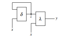Figure 1: Fully asynchronous Mealy machine

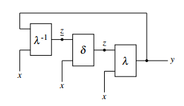Figure 2: Equivalent transformation
The following applies:
δ(z,x)= z

y mit y
The next stage of transformation shows at first sight no feedback. Only the RS-buffer, which is in δ, has a nested feedback. This transformation is outlined in figure 3. Transient states can be triggered via the input, while state stable states are being held via the RS-buffer. In order to set the correct state z to µ, the function δ must be well designed, which will be shown in the following sections.

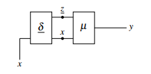Figure 3: Moore transformation
The following applies:
δ(z,x)= z µ(z,x)= y

2.1 Dual-rail logic

For the implementation in dual-rail logic [4], the fully asynchronous circuit from figure 1 will be divided in the 1- and 0-share. This is done by partitioning the state transfer function and the output function, see figure 4.

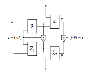Figure 4: Mealy realized in dual-rail logic
The functions δ and λ are each w.l.o.g. realized in two

blocks δ = (δz,δz) and λ = (λz,λz). In order to guarantee this secure dual rail structure, RS-buffers are used. The mode of operation corresponds in a certain manner to the Celement [4, 5]. The function δ of figure 3 will be designed by appropriate coding according to the RS-buffer, showing a general structure as outlined in figure 5.

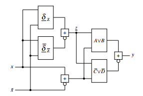Figure 5: Transformed Moore
The stabilized 1-states,c s ∆z c sz, are transformed into
1-outputs, Λyy. The corresponding Venn diagram of the stabilized 1-states in 1-outputs can be seen in figure

6. 1-states that appear as 0-outputs are declared as Λz, 0states which appear as 1-outputs are declared as Λz. The 1-partition is composed of:
Λy c sλy(δz)+λy(δz)+λy(δz)

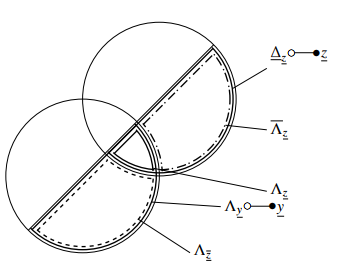Figure 6: Venn diagram of 1-states in 1-outputs

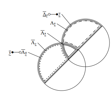Figure 7: Venn diagram of 0-states in 0-outputs
The stabilized 0-states,c s ∆z c sz, are transformed into
0-outputs, Λy y. The corresponding Venn diagram of the 0-states in 0-outputs is shown in figure 7. 0-states which appear as 1-outputs are declared as Λz, 1-states which ap-

pear as 0-outputs are declared as Λz. The 0-partition is composed of:

Λy c sλy(δz)+λy(δz)+λy(δz)
To understand the coding, first the RS-buffer has to be understood.

2.2 RS-Buffer

The RS-Buffer used and its circuit symbol are represented
in figure 8 and 9 and

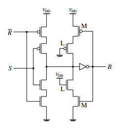Figure 8: RS-Buffer (schematic)

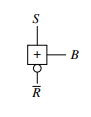Figure 9: Circuit symbol of the used RS-Buffer
its truth table is specified in table 1.
R 0 0 1 1
S 0 1 0 1
B B 1 0 B
Table 1: Truth table of the RS-Buffer
The RS-buffer is used to synchronize a dual-rail signal by only letting a state tranfer happen, if both incoming signals are disjoint (how it is desired) to each other. This means that there is no overlaying of signal, which could lead to fatal faults. The RS-buffer consists of the tri-state driver, which is the first state and the second stage the so called babysitter. The driving structure now provides 3 functions. Firstly the setting signal, which means the output is in the logical 1-state. Secondly the resetting signal, which means the output is in logical 0-state and least the hold state which holds the last state at the output by keeping the signal in the babysitter and having a high impedance state at the tri state. The babysitter consists of two complementary loops. The formula for the output B is therefore

B := R(B∨S)∨S(B∨R)= RS∨RB∨SB.

2.3 Design of the reduced state transfer function δ

As you can see the RS-buffer is coded via a 3-partitioning. There is the setting signal S=[1], the resetting signal R=[1] and the hold signal RS=[00]∨[11]. The state transfer function of an automaton can in turn be split in 4 parts. Firstly the transient……………..1-share, that means independent of the state the next state will be at logical 1, secondly the transient 0-share, that means output at logical 0 independent of the

state, thirdly the state stable share of the state transfer function, that means the share, which is at constant input dependent on the value of the last state and the state instable state, which means a permanent change of the state at constant input, see figure 10. The resulting 3 parts, which are left, can now be easily compared to the 3-partitition of the RS-buffer. The transient 1-share δ z is realized by the setting signal of the RS-buffer, similar the transient 0-share δ z is realized by the resetting signal and the state stable share is realized by the hold signal of the RS-buffer.

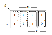Figure 10: Parts of a state transfer function
To understand the transformation, first a few compositions must be defined:
zδ(z,x)=δ(z = 1,x) zδ(z,x)=δ(z = 0,x) zδ(z,x)=δ(z = 1,x) zδ(z,x)=δ(z = 0,x)
This work only concentrates on function stable machines, so that state instable parts are not allowed. State instable parts can be deduced via

zδ ∧zδ
Functions must not exhibit these parts. The other parts can be deduced by the following expressions
transient 1 : δz = zδ ∧zδ transient 0 : δz = zδ ∧zδ state stable : zδ ∧zδ
This leads to the genereal formula for δi for n states:
δzi =δzi +¬δzi
=(ziδzi ∧ziδzi)+¬(ziδzi ∧ziδzi)
=(δzi(zi = 1,x)∧δzi(zi = 0,x))
+¬(δzi(zi = 1,x)∧δzi(zi = 0,x)) with i = 0…n−1

2.4 Design of the output function

The detailed description of the Venn-diagrams given in figure 11 and 12 is reported in [6].

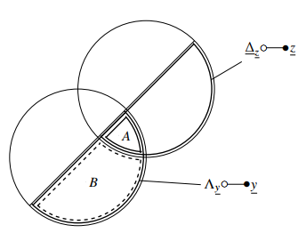Figure 11: Venn-diagram of 1-states in 1-outputs

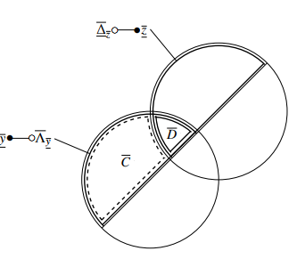Figure 12: Venn-diagram of 0-states in 0-outputs

The coding of the parts A, B, C and D of the Venndiagrams, see figure 11 and figure 12, is as follows:
(z,y)
(11)= A =δz ∧λy
(01)= B =δz ∧λy
(10)=C =δz ∧λy
(00)= D =δz ∧λy
The dual-rails y and y for y are now:
y = A∨B y =C∨D y = y+¬y
The seperate parts of the machine have now been deduced and can simply be strung together to get the form of figure5.

3. Use-Case

To get a better insight, three examples will be presented.
3.1 1-dimensional example
For x=(x1,x0), y=(y) and z=(z) the transformation of the Mealy machine (X,Y,Z,δ,λ) with the state transfer function and output function
δ(z,x)= x1x0 ∨zx1x0 λ(z,x)= x1x0 ∨zx1
will be executed. The automaton before the transformation can be seen in figure 13.

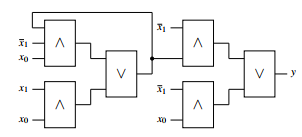Figure 13: Mealy machine before the transformation

3.1.1 Design of δ

The KV-diagram of the state transfer function can be seen in figure 14.

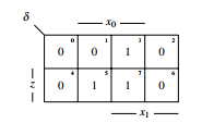Figure 14: The state transfer function
To code the RS-buffer correctly, firstly the KV-diagram will be compacted, see figure 15.

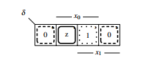Figure 15: Compacted KV-diagram of δ
The parts of the state transfer function can easily be seen and the KV-diagrams for δz and δz can be deployed, see figure 16. For δz 0 is coded as 1 and 1 is coded as 0 respectively, because of the dual-rail structure.

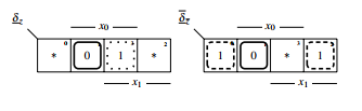Figure 16: δz and δz
For the next steps of the transformation, first the complement of δ has to be calculated:

δ(z,x)= zx1 ∨x0
The parts of the state transfer function are:
zδ =δ(z = 1,x)= x0 zδ =δ(z = 0,x)= x1x0 zδ =δ(z = 1,x)= x0
zδ =δ(z = 0,x)= x1 ∨x0
It has to be checked, if there are any instable parts: zδz ∧zδz = x1x0 ∧x0 = 0

zδ ∧zδ is 0 means the function has no instable parts.
The functions δz and δz can now be calculated via

The coding for δ of the RS-buffer is as follows:
(r s)
Set:(∗1)= x1x0 (transient……………..1-share)=δ z
Reset:(1∗)= x0 (transient 0-share)=δ z Hold:(∗∗)= x1x0 (state stable share)
Now δ can be derived:
δ =δz +¬δ
= x1x0 +¬(x0)

3.1.2 Design of λ

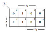Figure 17: Output function λ
The stabilized state transfer function has now been designed, now the output function must be designed. Therefore the output function has to be layed over the state transfer function and the parts have to be specified:

λ x 3.2 2-dimensional example
For x =(x1,x0), y =(y) and z =(z1,z0) the transformation of the Mealy machine (X,Y,Z,δ,λ) with the state transfer functions and output function
1 δz0(z,x)= x0 ∨z1x1 δz1(z,x)= z0x1x0 ∨z1x1x0
λ(z,x)= z1x1 ∨z0x1x0
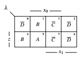Figure 18: Parts of the output function will be executed. The machine before the transformation is
The parts are:
A(z,x)= zx x x1
x0
B(z,x)= zx1x0 ∨zx1x0
C(z,x)= x1x0
D(z,x)= x1x0 ∨zx0 x1
x0
This leads to the output function:
x0 y = A∨B = x1x0 ∨zx1 y =C∨D = x1 ∨zx0
y = y+¬y = x1x0 ∨zx1 +¬(x1 ∨zx0) x1
The resulting automaton has the form of figure 19 with the
determined functions y = A∨B and y =C∨D. Figure 20: Automaton before the transformation

3.2.1 Design of δz0

δz
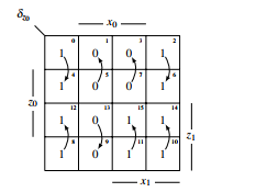Figure 21: KV-diagram of δz0
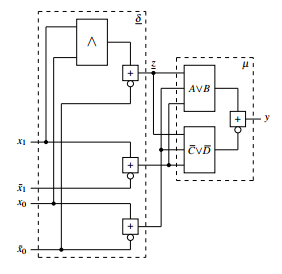Figure 19: Transformed Moore The KV-diagram of figure 21 will be lossless compacted given by the pointers in the diagram to the diagram of fig-
The truth table of the automaton: ure 22.
δz0
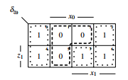Figure 22: compacted KV-diagram of δz0
With the compacted KV-diagram the RS-buffer for δz0
Table 2: Partial truth table of the resulting automaton can be coded by specifying the functions δz0 and δz0, see

figure 23. The partial function δz0 delivers the 1’s of δz0 as 1’s, while δzz0 delivers the 0’s of δz0 as 1’s. In this state transfer function, there is no state stable part only transient parts. Making the stable δz0 a normal dual-rail structure.

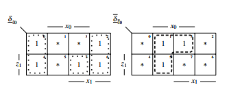Figure 23: δz0 and δz0
State instable parts are not allowed in the state transfer function:
z0δz0 ∧z0δz0 =(x0 ∨z1x1)∧(z1x0 ∨x1x0)= 0 Now the resulting z0 can be calculated:

z0 : =δz0 +¬(δ ) z0 : = x0 ∨z1x1 +¬(x1x0 ∨z1x1)

3.2.2 Design of δz1

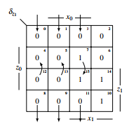Figure 24: KV-diagram of δz1
For δz1 the same approach applies. First the KV-diagram, see figure 24, will be compacted:

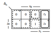Figure 25: compacted KV-diagram of δz1 Now the functions δz1 and δz1 can be deduced:

First δz1 is checked for instable parts:
z1δz1 ∧z1δz1 = z0x1x0 ∧(z0x0 ∨x1)= 0
No instable parts, so the RS-buffer can be coded for δz1 by

determining the functions δz1 and δz1:

z1 : =δz1 +¬(δ )
z1 : = z0x1x0 +¬(x1 ∨z0x0)

3.2.3 Design of λ

The KV-diagram of λ can be seen in 27. Because of the two-dimensional state, λ has to be divided into eight parts. They exist as follows:
(z1,z0,y) (z1,z0,y)
(001)= A (001)= E
(011)= B (011)= F
(101)=C (101)= G
(111)= D (111)= H

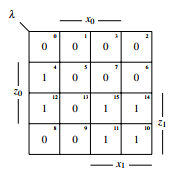Figure 27: KV-diagram of λ
The parts of λ are set up in the KV-diagram, see figure 28.

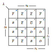Figure 28: Parts of λ
The output functions y and y can be inferred from this:
y = A∨B∨C∨D

y = E ∨F ∨G∨H

The resulting automaton can be seen in 30. As you can see in table 3, situation 7 leads to a cycle, by stepping to configuration 11, which steps back to configuration 7, and so on. So to have a state stable design in multistate machines, it is also necessary to regard the transitions between the states. A rule has to be found, to filter these race conditions. In the following transformation the auomaton of subsection b is stabilized, by changing δz1.

3.3 Stable 2-dimensional example

The state transfer function δz1 has now been changed, to make it a stable automaton. For x = (x1,x0), y = (y) and z = (z1,z0) the transformation of the Mealy machine (X,Y,Z,δ,λ) with the state transfer functions and output function
δz0(z,x)= x0 ∨z1x1 δz1(z,x)= z0x1x0 ∨z1x1 λ(z,x)= z1x1 ∨z0x1x0
will be executed. The machine before the transformation is outlined in figure 29.

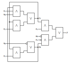Figure 29: Automaton before the transformation

3.3.1 Design of δz0

The KV-diagram of figure 31 will be lossless compacted given by the pointers in the diagram to the diagram of figure 32.

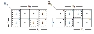Figure 33: δz0 and δz0

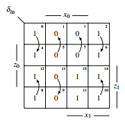Figure 31: KV-diagram of δz0

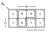Figure 32: compacted KV-diagram of δz0
With the compacted KV-diagram the RS-buffer for δz0 can be coded by specifying the functions δz0 and δz0, see figure 33.
State instable parts are not allowed in the state transfer function:
z0δz0 ∧z0δz0 =(x0 ∨z1x1)∧(z1x0 ∨x1x0)= 0 Now the resulting z0 can be calculated:

z0 : =δz0 +¬(δ ) z0 : = x0 ∨z1x1 +¬(x1x0 ∨z1x1)

3.3.2 Design of δz1

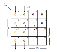Figure 34: KV-diagram of δz1

For δz1 the same approach applies. First the KV-diagram, see figure 34, will be compacted:

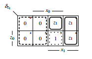Figure 35: compacted KV-diagram of δz1

First δz1 is checked for instable parts:
z1δz1 ∧z1δz1 = z0x1x0 ∧x1 = 0
No instable parts, so the RS-buffer can be coded for δz1 by

determining the functions δz1 and δz1:

z1 : =δz1 +¬(δz1) z1 : = z0x1x0 +¬(x1)

3.3.3 Design of λ

The KV-diagram of λ can be seen in 37. Because of the two-dimensional state, λ has to be divided into eight parts.
They exist as follows:
(z1,z0,y) (z1,z0,y)
(001)= A (001)= E
(011)= B (011)= F
(101)=C (101)= G
(111)= D (111)= H

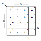Figure 37: KV-diagram of λ
The parts of λ are set up in the KV-diagram, see figure 38.

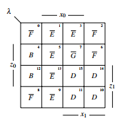Figure 38: Parts of λ
The output functions y and y can be inferred from this:

4. Test of Theory

To confirm the theory presented in the article, the state transfer function of the one dimensional example was analyzed making it a Medvedev. To simulate the circuit it was modelled with NAND gates and simulated in LT-Spice. The modeled NAND structure then was realized on the circuit board and the output was captured via an oszilloscope. The Medvedev machine (X,Y,Z,δ,1) with x =(x1,x0), y =(y) and z =(z) with the state transformation function and output function be given:
The KV-Diagramm:

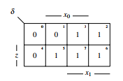Figure 40: KV-diagram of δ The table:

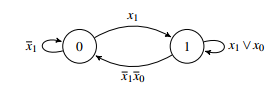Figure 41: Graph of the automaton
NAND gates have been used to realize the structure. Therefore the DNF was transformed into a NAND strucutre by twice negating the DNF.
δ(z,x)= zx0x1 ∨x1 = zx0x1 ∧x1

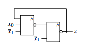Figure 42: machine before the transformation

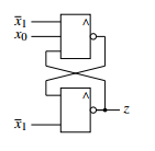Figure 43: Different view of the automaton
Figure 43 shows two asynchronous feedbacks, which can lead to a race. On transition of x1 from logical 1 to 0, while x0 stays on logical 1, the feedback, which is first on logical 0, will make the other to a stable logical 1. Therefore on this transition, it can not be forecasted, whether the output will be on logical 1 or 0.

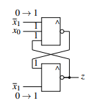Figure 44: Race condition

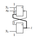Figure 45: Race z = 0

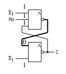Figure 46: Race z =1
To simulate the race condition, the circuit was modelled and simulated in LT Spice. The simulation shows a race.

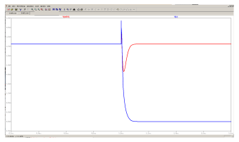Figure 47: Simulated race situation

The circuit was realized in reality and the race was captured via an oscilloscope.

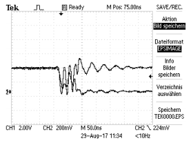Figure 48: Race situation in reality
Then the transformation, which was presented in this journal, was made leading to the following structure, which does not have any contending feedbacks anymore. The only feedback this structure needs is nested in the RS-Buffer.

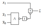Figure 49: Transformed Moore
This structure does not show a race problem. To prove this statement the race condition of the old automaton has been set to the inputs. In figure 50 the state z and the rising edge of x1 is shown. It’s clearly to see that the state doesn’t change, not even a fluctuation of the signal can be recognized. Therefore the transformed machine is determined and stable.

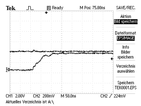Figure 50: Race condition applied to the transformed automaton

5. Conclusion and Future Work

An asynchronous function stable Mealy was transformed into a state stable Moore under the use of the RS-buffer with suitable coding. The transformation provides general asynchronous design rules, e.q. the isolation of critical situations via the hold function. Due to the stabilisation by RS-buffer with the hold function, no races will be propagated through the circuit. In this journal three examples have been presented, a 1-dimensional and two 2-dimensional. Although the stable 2-dimensional transformation has produced an asynchronous feedback, this feedback leads either to a confirmation or a hold of the RS-buffer. The feedback has to be seen as a starting condition which gets triggered by the input and a change of the feedback will only affect the RSbuffer if the input changes. This design guideline can be used for all circuit designs, to create a stable, reliable system. The goal of the design is to remove the outer feedback and nest it in the RS-buffer. The inputs have been coded as pseudo states and stabilized via the RS-buffer. The output function has also been designed in dual-rail. This leads to a circuit, that looks at first sight as a combinational circuit. With this method you can simplify complex automata and combine them. The results have to be simulated to get a detailed look at the behavior of the transformed Moore. As it was shown, one dimensional machines get stabilized by this design, but for more dimensional machines it is necessary to design stable functions and regard the transitions between the states, not only concentrating on one state. So a rule has to be found, which can check for instabilities between states and stabilize machines in these constellations. Additionally the formula for the Transformation can be programmed, to create an automated process of transformation. Additionally the output function λ has to be checked for functional Hazards and addapted to guarantee that they are no longer existing.

1. Birtwhistle, G.: Davis, A.: Asynchronous Digital Circuit Design, Springer London, 1995
2. Van Berkel, K.: Burgess, R.: Kessels, J.L.W.: Peeters, A.: Roncken, M.: Schalij, F.: A fully asynchronous low-power error corrector for the DCC player, IEEE J. Solid-State Circuits, vol. 29, Dec. 1994. – P. 1429-1439
3. Uygur, G.: Sattler, S.M.: A Real-World Model of Partially Defined Logic. 12th International Workshop on Boolean Problems 2016, Freiberg
4. Mokhov, A.: Khomenko, V.: Sokolov, D.: Yakovlev, A.: On Dual- Rail Control Logic for Enhanced Circuit Robustness, ACSD ’12 Proceedings of the 2012, 12th International Conference on Application of Concurrency to System Design, Pages 112-121, June 27 – 29, 2012, IEEE Computer Society Washington, DC, USA
5. Shirvani, P.: Mitra, S.: Ebergen, J.: Roncken,M.: DUDES: a fault abstraction and collapsing framework for asynchronous circuits, in Advanced Research in Asynchronous Circuits and Systems (ASYNC), Proceedings, Sixth International Symposium on, 2000, pp. 73–82
6. Özgül, M.: Deeg, F.: Sattler, S.M.: Mealy-to-Moore Transformation, 20th IEEE International Symposium on DDECS 2017, Dresden

(Click to view)

(Click to view)