1 Introduction

Designers face problems of two natures when building WLAN networks: issues that are inherent to radio resources’ planning and those concerning their integration with other network parts and upper-layer services in response to developing customers’ application needs such as mobility, real-time, interactive applications, business intelligence, and on-presence analytics. An accurate design should consider thoroughly both aspects and base its decision on a solid theoretical approach, on-field feedbacks, and best practices.

Design best practices dictate running two site surveys: one at the beginning of the project, before network’s deployment, and a second, after network’s deployment, to confirm resources’ planning results and to calibrate the system’s parameters in accordance to the real network’s condition. An optional survey may be required if radio environment or its utilization has changed and might affect the overall network capacity. The first survey qualifies mainly the exposure to on-reach foreign autonomous radio systems, and radio characteristics of the surface to cover (walls, floors, and other obstacles). The second site survey confirms the conformance of the actual deployment to design constraints in two ways:

1. by running a passive in-data-path survey that is based on passively reported statistics such as RSSI, SNR, PHY, MAC errors, packet count, etc. at radio interface level,
2. and an active one where in-data-path patterns simulate wireless client’s traffic classes to gather actively statistics on Jitter, RTT, or any other measure concerning the rendered service, application or experience.

This approach is not very accurate as it lies on a set of preconfigured unchangeable parameters that result from special case deployments and testing contexts, which may be completely different from the on-field reality. In the market-leading implementations such as Cisco TPC or Aruba ARM, we observe that at a certain point, a reference is made to an “ideal” preconfigured parameter. The third neighbor’s RSSI and a predefined hysteresis threshold [1] paremeters are used in the first case, and the “coverage index” [2] parameter in the second case, to decide on transmit power level planning network wide.

Inaccuracies come also from studies when they model the system as a pre-shaped radio coverage area in the form of a hierarchy of disks that delimit transmission ranges from interference or notalk ones. Some limitations arise also from no-sitesurvey techniques that base their radio resource management solely on WLAN reported measures. Other limitations come from simplifications such as to consider that a client association and the corresponding CSMA/CA mechanisms rely entirely on the strongest access point’s RSSI, because most of the interferences do not occur at MAC level, and radio measurements may differ from a vendor to another. Then it is necessary to ensure that model analysis inputs and outputs do not result in a contradiction.

Motivated by advances in beamforming techniques, especially from an array signal processing perspective, which make it possible to radiate energy in any direction and to easily estimate signal’s direction of arrival, this work solution model aims at fixing many of previous limitations by considering the opportunity for an access point to transmit in one specific direction. This opportunity processing accepts data from upper-layer services such as to achieve a complete end-to-end integration with other network parts.

As it will be demonstrated in this work, the number of transmit directions at access point level, could be optimized in conjunction with planning transmit power levels and channel assignment to maximize the overall network capacity. A cost-based approach prices in a timely manner each direction for an eventual transmission. Access points in this scheme discover each other over-the-air and report useful information on transmit directions, power levels and channels, to a central intelligence that coordinates the overall network operation. The ultimate result is:

1. Cancellation of co-channel interferences in a majority of deployment cases.
2. Processing of new transmission opportunities that are missing in conventional work.
3. Enhancement of end-to-end network performance.

In the upcoming section, we present a foundation on unified WIFI architectures and beamforming as they relate to this work. In Sect. 4, we discuss more formally the problem and in Sect. 5, we present our solution model. Sect. 6 discusses our solution results. In the end, we conclude and further our work. This paper is an extension of work originally presented in 2017 International Conference on Information Networking (ICOIN) [3].

2  Related Work

Co-channel interference in WLAN networks is a major problem that has been widely studied. To tackle this issue RRM and related techniques such as Transmit Power Control (TPC), Dynamic Channel Assignment (DCA), constitute a very accurate solution. If we consider TPC that is the focus of this work, the related-work’s approaches differ from each other in terms of the adopted interference’s model, inputs TPC may work on, and their processing (predictive, heuristic, etc.). We further focus on related-work’s adopted interference models.

To our knowledge, all models and derived TPC processing have considered only the transmission power level as a degree of freedom to limit co-channel interference. This work claims that the transmission direction could be an additional degree of freedom to overcome other models’ limitations when it comes to modeling irregular coverage areas in indoor WLAN environments.

Authors in this work [4] concentrate, from a lower layer perspective, on the co-channel interferences as a function of the estimated distance between the Access Points (AP) and the Wireless Devices (WD). In this scheme, the WDs estimate the distance based on the RSSI information sent by the APs in RTS control packets. The transmission power level adjusts accordingly to achieve a better network performance and interference cancellation. The issue with this model is that the power level adjustment affects other on reach WDs and APs communications. In addition, this model does not include cases where the WD does not simply receive the RTS packets.

In [5], a WD measures the amount of interference as a function of the local AP’s load, its signal’s strength and loads from the distant APs. Here interference is a linear function of the AP’s load. This is interesting but as opposed to our work, this model misses the interpretation of interference from an energy radiation perspective. In our work, we still include AP’s load consideration in the SLA applied to the processing of transmit opportunities.

Depending on the coverage area pattern: disks or Voronoi zones, the amount of interference in [6], is a function of different AP’s areas overlap in the first case and to their borders in the second one. This work model is very accurate to describe how an AP’s energy radiation could affect other neighboring APs. However, it is still insufficient to interpret many cases specific to indoor WLAN deployments that relate to onreach and unreachable AP’s. Subsection C of Sect. 4 discusses these cases in detail.

The authors in [7] consider both MAC and PHY layer inputs: data payload length, path loss condition, and frame retry counts, to find out the suitable PHY mode and power level combination. This procedure requires a control packet exchange that is similar to conventional RTC/CTS for this adaptation. This model is easy to implement but it is insufficient to interpret many cases specific to indoor WLAN similarly to the previous work. In addition and similarly to the first cited work, any PHY mode and corresponding power level change apply to all neighboring APs and WDs indistinguishably.

In [8], the authors concentrate on upper layer application performance such as FTP and HTTP, to find out an optimal power scheme or more exactly, an optimal combination between transmit power and supported load for a given distance between nodes. This model considers SLA as in the second and fourth cited works and augments its processing to include “behavioral” protocol aspects. However, the corresponding model misses the lower-level interpretation of AP’s radiated energy.

The authors in [9], approach the problem from an inter-protocol coordination point of view: WIFI, BT, etc. which may be very helpful to base an integratedsystem wide transmit decision or “etiquette” on the utilization of shared radio resources. In this scheme, all wireless devices broadcast the information on spectrum usage. This information includes transmit power level and frequency channel of use. In addition and based on costing policies, the system allocates resources: frequency, power and time, to wireless devices. This work is a generalization of the first and fourth previously cited works and may incur the same limitations.

In this work, we review the conventional cochannel wireless coverage models and show that the system could process more transmission opportunities and still conform to the SLA. In these works [4] [5], some of the transmission opportunities were missed in areas that were considered falsely as interference ranges or worst as no-talk ones. Our solution model considers inputs from upper-layer services to conform to the SLA on the end-to-end wireless client’s experience as in works [7] [8] [9]. In addition, it takes advantage of the technological advances in beamforming and related techniques, to introduce, at a conceptual level in indoor WLAN networks, the direction of transmission as a new radio resource added to frequency channel and power level, to enhance work’s like [9] results.

3 Theoretical Background

The next two subsections describe WIFI’s unified architecture in addition to the beamforming techniques as they relate to our study. The main objective of this foundation is to justify the feasibility of the hypotheses we base our study on. These hypotheses relate to the possibility to correlate reported radio interface’s information from different APs, to coordinate their operation network-wide, to concentrate the radiated energy in any direction, in a timely manner, and to estimate accurately the direction of known and unknown sources’ signals.

3.1         WIFI’s Unified Architecture

In dense indoor networks, the transmission is difficult to model and depends on radio environment’s characteristics such as obstacles, interference, background noise, density of wireless clients, mobility applications, etc.

In this context, standalone APs’ architectures do not scale with high number of APs and WDs that require high class QoS treatment. Such architectures are replaced gradually by controller-based or “unified” ones. They are marked as unified for two reasons:

1. a central decision-making and intelligence, that is a Wireless LAN Controller (WLC), manages the overall network’s operation.
2. the WLAN integrates with the overall network parts: LAN, WAN, DCN, etc. from especially a QoS perspective.

The market-leading vendors implement such a central decision-making processor mainly in three ways:

1. appliance WLC-based,
2. virtual system WLC-based,
3. distributed AP-based.

In the latter implementation, the APs take over the

WLC’s role. The first two implementations require a WLC, a virtual or physical appliance, which is reachable by all network APs over the wire. Examples of such WLCs are Cisco 8540 Wireless Controller and Aruba 7280 Mobility Controller.

Cisco unified architecture [10] defines two protocols:

1. CAPWAP, used by APs to build protocol associations to the active WLC.
2. NDP, to send messages over the air (OTA) for APs to exchange proprietary and standard management or control information.

In addition to these protocols, Cisco APs integrate a set of on-chip RRM techniques: CLIENTLINK and CLEANAIR that monitor and measure radio environment characteristics among other features. The WLC gathers this information via the already established CAPWAP tunnels to APs. Further, platforms such as Cisco Prime Infrastructure (CPI) and Mobility Services Engine (MSE) extend the capability of CLEANAIR to perform analytics, locate clients, interferers, and build heat maps. Based on the APs’ reported information, the WLC computes the channel assignment and power levels map network wide. Its decision still conforms to the pre-configured policy sets. Each of these sets defines a number of configurable variables and unchangeable settings such as acceptable signal levels, tolerable noise levels, usable power levels, frequencies and channels, etc.

In this work context, the WIFI unified architecture guarantees a coordinated operation between all network elements at a very low level, an accessible distributed intelligence, and a centralized decisionmaking. It focuses on how to enhance the centralized decision-making at WLC level and especially RRM processing. RRM is the set of tools, algorithms and services that processes inputs from AP’s radio and LAN interfaces and outputs a wireless area coverage plan or map that conforms to a predefined utility function.

3.2         Beamforming

The majority of WLAN communicating systems are equipped with omnidirectional antennas or a set of limited number of unidirectional antennas to obtain an equivalent energy radiation’s pattern. Ease and cost of such hardware configurations are some of the benefits of such designs but they lack many aspects regarding interference and noise cancellation, signal sources’ localization, and power consumption.

Beamforming techniques by definition relate to both the direction of energy radiation and the estimation of signal’s arrival direction [11] and from an array signal processing perspective, they offer the possibility to tackle previous issues and design limitations to the next level in three ways:

1. the radiation of energy toward actual receivers allows better performance and less impact on the other system’s elements.
2. the estimation of direction of known and unknown sources allows better costing of a given directed transmission.
3. the on-chip beamforming techniques allows for a hardware real-time adaptation to extremely changing radio environments like in our context.

With reference to [11], beamforming concerns both sides of a communicating system: the emitter and the receiver. It allows the radiated energy to be concentrated in one direction and to estimate its corresponding source’s location for both legitimate and rogue interferers at receiver level. Basically, beamforming could be achieved mechanically by manually or electronically gearing a directional antenna. From a signal processing perspective, beamforming is achieved by changing certain transmitter’s characteristics such as array elements’ phase shifting, source signals’ amplitude increasing or addition weighting. Additionally, the desired array gain and beam’s direction depend on the number and geometry of array elements.

To ease our study we consider that array beamformers achieve equivalent performance to mechanical ones concerning both the resultant beam radiation’s angle and signal’s gain.

Let us consider an antenna with a beamwidth of 2 ∗ θ_n such as the radiated energy in the zone delimited by this angle is equal to the maximum energy radiated by the antenna minus n dB. n is calculated in such manner to allow an AP to transmit in all corresponding directions at the same time without interfering with each other. A rough estimation of this number is:

                                   N ≈ (2 ∗ π)/ (2 ∗ θ_n)                              (1)

In the contexts of [12] [13] studies on antenna arrays, the beamwidth is expressed as a function of the distance between array elements d, the number of elements M, and the wave length λ:

                                ∆θ_main ^≈ (2 ^∗ λ)/ (d ^∗ M)                           (2)

In general, the evolving antenna array’s beamformers could be classified as data independent, statistically optimum, adaptative or partially adaptative [11]. In this work, data dependent data beamformers (statistically optimum and adaptative) are of interest. Some of these beamformers are Multiple Sidelobe Canceller (MSC), Reference Signal (RS), Max SNR, Linearly Constrained Minimum Variance

(LCMV), Lean Mean Square (LMS), Recursive Least Squares (RLS).

The other part of beamforming relates to the estimation of the Direction of Arrival (DOA). DOA estimation methods may include Bartlett, Capon, MUSIC, Min-Norm, DML, SML, WSF, Root-Music, ESPRIT, IQML, and Root-WSF. SML, WSF and Root-WSF are statistically the most efficient depending on the array geometry [14]. They could be yield into two main categories: spectral-based techniques, which are computationally optimal, and parametric methods, which are more accurate than the previous ones.

Recent algorithms are more accurate in the estimation of signal’s arrival of both known and unknown sources. They depend on the array size, antenna’s radiation pattern, source signals’ correlation, data statistics, corresponding data generation framework, among others. However, for the rest of this study we could consider that beamforming techniques allow:

1. sufficient number of directions to mimic an omnidirectional operation,
2. geographically any direction is achievable,
3. patterns from different directions at the same AP level do not interfere and are uncorrelated,
4. on-chip real-time transmits and synchronization.

4  Problem Statement

In this section, we formalize mathematically the problem of determining the opportunity to transmit at any point under the wireless coverage area. We first focus on related-work’s models. Then in the next sections, we present our solution model and compare its results to preceding studies.

In this problem statement, we focus mainly on how related-work estimates the interference at a given point under the wireless coverage area, applies radio and upper-layer constraints, and processes the corresponding transmit opportunity.

To ease this work we consider the wireless coverage area as a two-dimensional Euclidean plane. The APs and WDs are points of this plane. They transmit in the same channel and cause the majority of co-channel interference in this area. This study focuses on co-channel operation but is easily extendible to tackle cross-channel interference or noise issues in the context described before. Let us define:

{AP₁,AP₂,…,AP_n}— set of n access points.

P_j               — a point under wireless coverage area.

(x_i,y_i)— coordinates of AP_i or P_i points in an Euclidean two-dimensional plane.

w_i,w_min,w_max,w_opt— AP_i’s    corresponding      current, minimum, maximum and optimum transmit power levels.

d_i,j               — distance between AP_i and P_j points.

I(),O()— interference         and         transmit opportunity functions.

We categorize related-work’s models into two categories: Range-based and Zone-based. In the upcoming subsections, we describe each of them and discuss their limitations.

4.1         Range-based Model

In works similar to [4], an AP’s wireless coverage corresponds to one of these ranges: a transmission, interference or no-talk range. These ranges correspond to the estimation of the distance between the AP and a receiving point P (AP or WD). Further, they consider that an AP’s wireless coverage pattern is omnidirectional in the form of a circle or a disk. In this configuration, the three circles that correspond to each range type and centered at the AP define the whole AP’s wireless coverage area as in Figure 1.

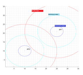Figure 1: Range-based model’s representation of an AP’s wireless coverage

Let us further define:

C_i,tx,C_i,if ,C_i,nt— AP_i attached circles that delimit corresponding transmission, interference and no-talk ranges.

R_i,tx,R_i,if ,R_i,nt— AP_i corresponding ranges.

If we suppose that:

                                       Ri,tx ≤ Ri,if ≤ Ri,nt                                                   (3)

Then the interference and transmit opportunity are given as follows:

                    X3              X

I(Pi) ≈           αk                   βj ∗ intersection(Cj,k,Ci,1) k=1             j,i	(4)
1 O(Pi) ≈ 3 P P ∗ intersection(Cj,Pi) αk βj	(5)

                      k=1           j,i

A weighted version of these functions is given further to account for inaccuracies and other constraints. The α and β weights are meant to reflect the nonlinearity of interference addition, the power level’s effect on interference strength, and the type of transmission’s range. Here we consider that the interference at a given point P_i is a function of other AP_j’s signals except from the AP_i to which the point is associated. The opportunity processing is slightly different as it considers all AP’s interference to P_i that is not associated to any AP_i yet.

4.2    Zone-based Model

Works such as [5] [6] that are based on this model are different from the previous ones as ranges here are not function only of the corresponding AP transmission’s characteristics: channel, power level, etc., but depend also on the neighboring APs. The result of this is that the transmission range shape is no more a solid circle but a convex polygon with straight sides. Each straight side defines a borderline that separate two neighboring APs’ transmission ranges. Consequently, it is important to note that a point in a transmission range of one AP could not be in another AP’s transmission range. A Zone-based AP’s wireless coverage is represented in Figure 2.

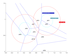Figure 2: Zone-based model’s representation of an AP’s wireless coverage

Let us further define:

G_i — AP_i corresponding transmission range polygon or zone.

Then the interference and transmit opportunity are given as follows:

               I(P_i) ^≈ α₁^Xβ_j ^∗ intersection(C_j,1,C_i,1)^−λ                                  (6)

^P α_k ^P β_j ^∗ intersection(C_j,k,G_i) k=2 j,i

Similarly to formulas 4 and 5, α and β weights are meant to represent the impact of AP’s transmission characteristics. λ is representative of the neighboring APs impact on AP_i borderlines. In this configuration, only transmission range is affected. The processing of other ranges are the same as in the previous model. It is also to note that opportunity in this model correspond to P_i in AP_i transmission’s range or zone G_i rather than intersection of the neighboring APs like in the previous model.

4.3         First Observations

The presented models’ functions of interference and opportunity do not reflect the accuracy of interference and opportunity measurements but rather the concept behind them and their possibilities to account for different WLAN design cases and aspects. At this stage, we see clearly that both models are limited in these ways:

1. both models are limited to consider that the strength of interference is only inversely proportional to the distance of an AP from interfering neighbors.
2. both models would interpret an increase in a transmission power level as an expanded reach in all directions: uniformly in case of Rangebased models but depending on neighboring APs in case of Zone-based ones.
3. a point could not be in two transmission ranges of two different APs at the same time in Zonebased models.
4. transmission range does not depend on the strength of interference in Range-based models.
5. both models would interpret falsely obstacles to the signal propagation, as a weaker signal from an AP in the context of indoor WLAN networks does not mean necessarily that this AP is out of reach.
6. similarly to the previous point a stronger signal does not mean necessarily that an AP is in reach: it signal may be guided under some conditions.

The consequence of these limitations in indoor WLAN networks, is to reduce or overestimate the transmit opportunities that the network may offer. The upcoming section presents our solution to fix these modelization limitations.

5. Solution model

Our solution model is suitable for WLC-controlled indoor networks in the already explained conditions. For the purpose of this study, we suppose that APs are equivalent, support MIMO technologies such as beamforming and DOA, and operate over the same channel. The wireless devices (WD) are equipped with omnidirectional antennas and transmit at a lowered power level in comparison with APs. The model runs three algorithms:

1. Transmit Direction Discovery (TDD) algorithm that builds a per direction neighbor discovery map, computes the optimal number of transmit directions and the corresponding per direction power levels.
2. Transmit Direction Mapping (TDM) algorithm estimates the impact that may have an AP on the network when it transmits in a specific direction and builds consequently, a per-direction transmit cost-based map that represents this information.
3. Transmit Direction Opportunity (TDO) algorithm processes data from both TDM and the upper-layer network services to optimize the transmission opportunities and build a perdirection transmit opportunity-based map to represent this information.

The next workflow in Figure ?? is an overview of our solution processing.

At initialization, the number of transmission directions is set to the minimum and the power level to the maximum. TDD processing stops after all APs are discovered and exactly one or no neighbor AP is discovered at any AP direction.

Based on results from TDD, TDM categorizes the coverage area points and costs a potential transmission at each of them. The coverage area points belong to one of these three categories: Not-OnAny-Transmit-Direction (NOATD), On-Discovered-

Neighbor-Direction (ODND), and Not-ODND-On-

Transmit-Direction (NOOTD). After the coverage area point’s categorization, the system processes the transmission costs.

TDO algorithm evaluates the opportunity to transmit at a specific coverage area point. It returns the AP that may handle the transmission and the corresponding direction. This processing accepts inputs from TDM and the upper-layer SLA. The SLA processing is tight to the AP’s wired network interface as opposed to the radio interface.

5.1         TDD algorithm

TDD algorithm processes the optimal number of transmission directions that APs may support and the corresponding per-direction transmit power levels. To ease this study, we consider these hypotheses and simplifications:

1. only a 2D plane operation is considered.
2. a uniform beamwidth in all directions.
3. APs are able to achieve an emulated omnidirectional operation.
4. two signals from the same AP in two different directions could not interfere.
5. all APs have the same optimal and maximal numbers of transmission directions and corresponding power levels.
6. neighbor discovery is bidirectional, occurs at the opposite direction, and at the same transmit power level.
7. an AP could not discover the same neighbor AP in two separate directions.
8. an AP could not discover itself.
9. at least one neighbor AP is reachable in any AP direction.

Points 2, 3, 4 and 5 are idealistic physical characteristics of AP’s beamforming implementation. The 9^th point indicates that a co-channel interference condition is detected from a neighboring AP. The 6^th, 7^th and 8^th assumptions are further developed in separate work to cover and interpret cases where:

1. the optimal numbers of transmission directions and power levels are not the same among APs.
2. neighbor discovery is unidirectional or asymmetric.

Let us define:

(d_i,w_i)— the direction and power level associated with AP_i.

d_−j(−x,−y)— the opposite direction of d_j(x,y) in an euclidean 2D plane.

L(AP_i,d_j,w_k)— the segment that represents the transmission range of AP_i in d_j direction at w_k transmit power level.

a(i,j), b(i,j), c(i,j)— respectively         the          segment L() slope, intercept and end point.

X(AP_i,d_j,w_k)— the set of discovered AP neighbors by AP_i in d_j direction at w_k power level.

O(AP_i,AP_j)— a segment that represents an obstacle between AP_i and AP_j.

We formalize the problem as:

∀i ∈ N,                                                                                       (8)

               ^∃j,k ^∈ _N s. t.           X(AP_i,d_j,w_k) , ^∅

^∀i,j,k ^{∈ N},                                                                                  (9)

AP_i < X(AP_i,d_j,w_k)

^∀i,j,j⁰,k,k^{0 ∈} _N,              and      j , j⁰,                                     (10)

X(APi,dj,wk) ∩ X(APi,dj0,wk0 ) = ∅

^∀i,i⁰,j,j⁰,k,k^{0 ∈} _N,               and      i , i⁰,                                 (11)

APi0 ∈ X(APi,dj,wk) ≡ APi ∈ X(APi0 ,dj0 ,wk0 )

        and      dj0 = d−j,       wk = wk0

^∀i,j ^∈ _N,                                                                                   (12)

                                  n                                     h                  io

                L(APi,dj) = ai,j ∗ x +bi,j             |       x ∈ xi,xi +ci,j

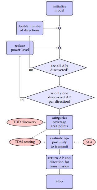Figure 3: Flowchart of our solution model processing

The APs’ distribution on the plan could be any random function or resulting from on-site surveys. However, we consider that the minimum and maximum distances between any of these APs are linear functions respectively of the corresponding minimum and maximum supported power levels. Figure 4 represents a simple network of seven APs with eight transmission directions each. Eight beams in red color are formed roughly around AP_i corresponding transmission directions.

The AP neighbor’s per-direction discovery is based on the distance between APs that are on each other theoretical transmission range, on-site surveys, and radio interface sensing. Additionally the solution model allows the discovery of these two design special-case neighbors:

1. “isolated” neighbor AP that is at reach but separated by an obstacle.
2. “guided” neighbor AP that is not at reach but received with an acceptable signal level.

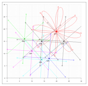Figure 4: TDD Discovery Map example of 7 APs and

8 transmit directions

With reference to Figure 4 network’s representation, the results of neighbor AP’s discovery are given in Table. 1.

Table 1: Neighbor AP’s discovery results

AP	d1	d2	d3,	d4	d5	d6	d7	d8
AP1	AP6	∅	∅	∅	∅	∅	AP2	∅
AP2	AP5	AP6	AP1	∅	∅	∅	AP6	∅
AP3	∅	∅	AP7	AP6	∅	AP5	∅	∅
AP4	∅	∅	∅	∅	AP6	∅	AP7	∅
AP5	∅	AP3	∅	∅	AP2	∅	∅	∅
AP6	AP7	AP4	∅	∅	AP1	AP2	∅	AP3
AP7	∅	∅	AP4	∅	AP6	∅	AP7	∅

The optimization of APs transmission directions’ number is a three-step process. For directions with more than one discovered neighbor, we calculate a new number such as to have the least possible number of neighbors per any AP’s direction. Otherwise, we adjust the power levels to get some of these APs out of reach from the local AP. If no success, we revert to Range-based-like interference scheme to cost this transmission zone.

A simpler form of the proposed algorithm is given next:

1: (dopt,wopt) ← (dmin,wmax)

                  Sopt                              max,wopt)

2: X ←             j=1X(APi,dj

3: for j = 1 to opt do

4:                                          if opt ≤ max then opt

5:                if card(X(AP_i^,d_j              ,w_opt)) > 1 then

6:                   dopt ^← d2∗opt

7:                                              end if opt

8:             else if card(X(AP_i,d_j              ,w_opt)) > 1 then

9:                    repeat Sopt     opt

10:                 if        j=1X(APi,dj              ,wopt−1) = X then

11:                      wopt ^← wopt−1

12:                                                           end if opt

13:             until ∀j,        card(X(AP_i,d_j            ,w_opt)) ≤ 1

14:        end if

15: end for

The optimum numbers of directions and power levels are respectively initialized to the minimum and the maximum numbers supported by AP_i. For every AP’s direction, we check the number of discovered neighbors. If many neighbors are detected, we multiply the initial number of directions by two until we obtain only one neighbor per direction. If the maximum number of direction is reached then we reduce by one level the power and try to get the same result without altering X. X is the set of all neighboring APs that were detected previously in the maximum supported directions and at the maximum supported power level.

5.2         TDM algorithm

In the previous section, TDD returned the optimal number of transmission directions, the corresponding optimal number of power levels and the sets of AP’s per-direction discovered neighbors. In addition to these elements, TDD interprets the presence of two kinds of obstacles: those that are preventing isolated neighbors from seeing each other, and those that are creating new transmission opportunities among guided neighbors. One way for TDD to interpret such kind of obstacles is by comparing the on-theair discovery’s results with on-site surveys’ information. Based on the previous elements, TDM algorithm builds a transmission-costing map for APs to reach any point under the overall wireless coverage area.

A simpler form of the proposed algorithm is given next:

1: for j = 1 to opt do

2:                if P_i ∈ L(AP_i,d_j) and X(AP_i,d_j) , ∅ then

3:              Case₁

4:                else if P_i ∈ L(AP_i,d_j) and X(AP_i,d_j) = ∅ then

5:              Case₂

6:          else

7:              Case₃

8:          end if

9: end for

TDM costing system categorizes WDs as NOATD, ODND, or NOOTD. These WDs could be represented roughly by circles with sufficiently small radii in comparison with APs transmit ranges, to not false processing results. We process carefully NOOTD points, which are not on discovered-neighbor APs’ directions, as they are hard to detect. Let us define:

C_i^W D— WD attached circle.

ρ_i               — weights associated with each category.

Cost(P_i)— function of transmissions cost at P_i

Then for this preliminary work, the cost of a transmission could be expressed as follows:

 ρ1I(Pi),   Cost(Pi) ≈  ρ2I(Pi),    ρ3I(Pi), Where,	if if if	NOAT D ODND NOOT D	(13)
XX I(Pi) ≈ α1             βj,k ∗ intersection(Lj,k,CiWD)			(14)

                        j         k

3

                       X          X

                 +        α_k                  β_j ∗ intersection(C_j,k,C_i,1)

                     k=2             j,i

Cost calculation results were plotted on Figure 5, for the same Figure 4 network example set of seven APs and eight transmission directions. On this map, transmission costs range from white color, lowest cost points, to red color that correspond to the highest costly points.

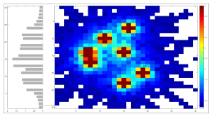Figure 5: TDM Cost Map example of 7 APs and 8 transmit directions

5.3         TDO algorithm

TDO takes into consideration the worst-case analysis done by TDM when all the APs transmit at the same time in all supported directions at the maximum power level. Then for a given transmission, it prioritizes the directions with the least cost in duality with TDM but in addition, it integrates data from the upper service layers and returned SLA tests both on the passive and active communication’s paths.

A more complex form of this opportunity processing relies on a system-wide APs transmit operation’s synchronization to cancel costly directions and onthe-air tests to optimize NOOTD costs. Let us define:

s_1,i,s_2,i— AP_i weights associated with defined SLA passive and active test results.

O(P_i)— opportunity of transmission function at P_i.

Then for this preliminary work, the transmission opportunity calculation at any point P_i is given by:

                          O(Pi) = s1,is2,iI(Pi)                                          (15)

The transmission opportunity processing results were plotted on Figure 6 for a set of seven APs and eight transmit directions.

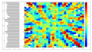Figure 6: TDO Opportunity Map example of 7 APs and 8 transmit directions

s_1,i and s_2,i weights are calculated based on the simulated SLA active test results that may include: Packet Loss Rate, Round-Trip Time (RTT), Jitter, and on SLA passive measurements at PHY and MAC levels like: error rates, transmitted packets, etc. that are directly taken from the radio and LAN interfaces. In addition, these weights take into consideration the nature of the end-user application: real-time applications do not require the same service from the network as bulk ones.

5.4   Layered Transmit Opportunity Processing

With regard to this work opportunity processing, a transmission is a four-step procedure: discover, cost, evaluate, and transmit. Discovery is primarily done by APs and could be extended to any WD. The interpretation of discovery results, costing, and opportunity processing, are done at WLC level. Costing in this work has been solely based on interference estimation but could integrate any other radio interface’s measurements: Signal to Noise Ratio (SNR), Received Channel Power Indicator (RCPI), and so on. Opportunity evaluation is based both on previous radio interface costing and on measures from upper layer services. These two measures have to be fully uncorrelated to not false results.

5.5  Transmit Synchronization

In this configuration, a transmission is not tight to the access point WD is associated with, but rather to the AP that offers the best transmit opportunity among a set of APs. In fact, the WD is associated with a virtual or pseudo AP that is representative of a set of physical APs with common characteristics with regard to this association. Any physical AP attached to the pseudoAP could source an effective transmission to the associated WD. In the context of this work, we match the

WD’s corresponding pseudo-AP to a single physical AP.

6. Evaluation and Conclusion

At this stage, the evaluation is based on Matlab simulations of both our model and models from relatedwork [4] [5] [8] Range-based, and [6] Zone-based solutions. In the next step, we consider implementing this solution on a Linux-based APs and WDs and compare its performance with simulated related-work and vendor’s implementations.

We compare our model performance to both Range-based and Zone-based models in these three transmission conditions:

1. a free space transmission condition,
2. the presence of obstacles, “isolated” neighbor’s condition,
3. “guided” neighbor’s condition.

We first evaluate the compared transmission opportunity for any set of 30 APs and ten times a randomly selected 100 WDs on a 2D grid. To ease this work we limit the maximum number of APs to 30 and the number of WDs test points to 100.

Figure 7 shows that for 30 APs and 10 random sets of 100 WDs on the grid, the average performance calculations is almost: 77% for our solution, 68% for Zone-based and only 57% for Range-based models. Figure 8 shows the average transmit opportunity for each model per WDs sets.

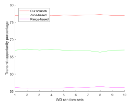Figure 7: Performance comparison for 30 AP and 10 random sets of 100 WDs

Second, as in Figure 9, we evaluate the APs number impact on the compared performance for any set of 100 WDs. APs number ranges from 1 to 30. In Figure 10, we compare Zone-based to Range-based models.

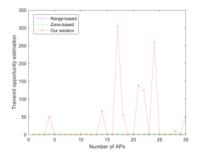Figure 9: Comparison of our solution, Zone and Range-based models for any set of 100 WDs by APs number

We see clearly that our solution is comparable to Zone-based one when α is almost 75%. Our solution is near optimal when α is 12,5% but this is idealistic. However, achieving a 50% α is realistic with regards to these-days vendors APs system characteristics. A 50% α coefficient may correspond roughly to Conflict of Interest The authors declare no conflict four transmission directions or beams. of interest.

Acknowledgment

We would thank colleagues : researchers, engineers, and anonymous reviewers for sharing their precious comments and on-field experience that improved the quality of this paper.

1. “Radio Resource Management White Paper.” [Online]. Available: https://www.cisco.com/c/en/us/td/docswireless/controller/technotes/8-3/b RRM White Paper.html
2. “ARM Coverage and Interference Metrics.” [Online]. Available: http://www.arubanetworks.com/techdocs/ArubaOS 64x WebHelp/Content/ArubaFrameStyles/ARM/ARM Metrics.htm
3. M. Guessous and L. Zenkouar, “Cognitive directional costbased transmit power control in ieee 802.11 wlan,” in Information Networking (ICOIN), 2017 International Conference on. IEEE, 2017, pp. 281–287.
4. R. Ruslan and T.-C. Wan, “Cognitive radio-based power adjustment for wi-fi,” in TENCON 2009-2009 IEEE Region 10 Conference. IEEE, 2009, pp. 1–5.
5. N. Ahmed and S. Keshav, “A successive refinement approach to wireless infrastructure network deployment,” in Wireless Communications and Networking Conference, 2006. WCNC 2006. IEEE, vol. 1. IEEE, 2006, pp. 511–519.
6. R. Prateek and P. Om, “Interference-constrained wireless coverage in a protocol model,” in Proceedings of the 9th ACM international symposium on Modeling analysis and simulation of wireless and mobile systems Terromolinos, Spain: ACM, 2006.
7. A. Akella, G. Judd, S. Seshan, and P. Steenkiste, “Selfmanagement in chaotic wireless deployments,” Wireless Networks, vol. 13, no. 6, pp. 737–755, 2007.
8. D. Qiao, S. Choi, A. Jain, and K. G. Shin, “Adaptive transmit power control in ieee 802.11 a wireless lans,” in Vehicular Technology Conference, 2003. VTC 2003-Spring. The 57th IEEE Semiannual, vol. 1. IEEE, 2003, pp. 433–437.
9. D. Raychaudhuri and X. Jing, “A spectrum etiquette protocol for efficient coordination of radio devices in unlicensed bands,” in Personal, Indoor and Mobile Radio Communications, 2003. PIMRC 2003. 14th IEEE Proceedings on, vol. 1. IEEE, 2003, pp. 172–176.
10. “Enterprise Mobility 8.1 Design Guide.” [Online]. Available: https://www.cisco.com/c/en/us/td/docs/wireless/controller/8-1/Enterprise-Mobility-8-1-Design-Guide/Enterprise Mobility 8-1 Deployment Guide.html
11. B. D. Van Veen and K. M. Buckley, “Beamforming: A versatile approach to spatial filtering,” IEEE assp magazine, vol. 5, no. 2, pp. 4–24, 1988.
12. V. Rabinovich and N. Alexandrov, “Typical array geometries and basic beam steering methods,” in Antenna Arrays and Automotive Applications. Springer, 2013, pp. 23–54.
13. T. C. Cheston and J. Frank, “Phased array radar antennas,” Radar Handbook, pp. 7–1, 1990.
14. H. Krim and M. Viberg, “Two decades of array signal processing research: the parametric approach,” IEEE signal processing magazine, vol. 13, no. 4, pp. 67–94, 1996.

(Click to view)

(Click to view)