1. Introduction

As radios in future wireless systems become more flexible and reconfigurable and available radio spectrum becomes scarce, there is the possibility of using TV white space devices (WSDs) as secondary users in the Broadcast Bands without causing harmful interference to licensed incumbents. Currently, one candidate method could be to utilise a geolocation database approach. The white space device should be able to determine available channel opportunities for a given location by accessing a database of TV White Space (TVWS) channels including data on each transmitter and each site, variable channels, transmitter power, and time of validation [1]. Therefore, the TV channel can be protected from harmful interference by accurate prediction of TVWS using an appropriate propagation model. Design of any wireless network depends on accurate prediction of radio propagation, which impacts deployment and management strategies. In this paper we extended the previous work by investigating the best propagation model among three propagation models (Extended-Hata, Davidson-Hata and Egli), using various terrain data resolutions (1000, 100 and 30 m) and comparing with the real measurements taken around Hull UK using two the performance comparison criteria of implementation time and accuracy. Agreement between the measured and predicted values of path loss has investigated, using MATLAB to analyse and compare the variation of path loss between the measured and predicted values. The terrain profile was extracted from terrain database Global1 and then taken into account in selected propagation models. The flexible cognitive TVWS database system was built using different propagation models to calculate available channels in each pixel of the selected area.

2.       Digital Terrain Elevation Data (DTED)

DTED was developed by the US Defense Mapping Agency (DMA) and can be used to improve signal detection accuracy. Currently, the paper has selected only three DTED levels of spatial resolution, which are available to the public [2].

Table 1: Resolution levels of DTED.

DTED Level

Post Spacing

Ground Dist

Row x Column

0	30 arcsecond	~ 1 km	121 x 121
1	3.0 arcsecond	~ 100m	1200 x 1200
2	1.0 arcsecond	~ 30 m	3600 x 3600

The elevation data of the resolution from 30 arcsecond (arcsec) to 1 arcsec (level 0,1 and 2 ) are avaliable for public use and can be downloaded as different DTED extension files in each resolution. The USGS web application has been used to define the desired research region by specifying latitude and longitude as shown in Figure 1, which identifies the required terrain tiles. Figure 2 classifies all tiles, identified by the web application  earthexplorer.usgs.gov .

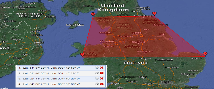Figure 1. Region selected for terrain data acquisition

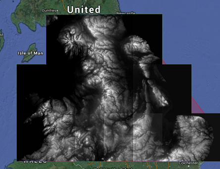Figure 2. Research region of terrain elevation data by NASA’s shuttle radar topography mission (SRTM) with resolution 1 arc sec (30 m)

3.       TVWS Geolocation Database

The use of a TV white space geolocation database enables the most effective detection method for prediction of available channels and calculation of TV coverage maps for each pixel in the selected region by using an appropriate propagation model, selected for accuracy and efficiency. The technique can avoid signal detection problems caused by fading effects and shadowing. Construction of the geolocation database requires primary user information including frequency of operation, transmitted power, location, transmission time and height and type of transmit antenna. This information will protect spectrum incumbents from interference from secondary users who will access the database by sending a query to obtain available channels in a given area at a certain time. Furthermore, the geolocation database might have proxy to make queries and identify available channels for WSD [3].

4.       Propagation Models

When planning wireless communication systems and designing wireless networks, the accuracy of the prediction of propagation characteristics of each environment should be taken into account. One of the most significant parameters, which can be provided by propagation prediction, is large-scale path loss, which affects directly the coverage of a base station placement and its performance. However, using field measurements to obtain these parameters without depending on propagation models is time-consuming and costly. The following subsections provide a brief explanation of several appropriate empirical propagation models [4] including the Extended Hata, Davidson-Hata and Egli models.

4.1.  Extended Hata Model

The Extended Hata model was derived from Hata-Okumura which is widely used for signal prediction in urban areas, wholly based on measured data that have been collected in Tokyo Japan. Also, it does not have any analytical explanation, but includes empirical factors that depend on the type of environment. This model can be used in different environment by adding some correction factors to meet the requirements of ITU-R and also extending range up to 100 km as shown in the following equation:

Where represents the carrier frequency (150 to 1500 MHz),  is the height of the base station antenna (m) and is the height of receive antenna (m). The distance from transmitter to receiver is d km. The value of the correction factors a( ) and C depend on the type of environment. In small and medium sized cities and metropolitan areas the value of C will be 0, while in other environments such as suburban and rural areas, different equations are used [5]. The factor b denotes an extended range up to 100 km as shown in the following equation.

4.2.  Davidson-Hata Model

This model is based on modification of several corrections to Hata’s formulas for extending the distance up to 300 km and the frequency range from 30 to 1500 MHz as mentioned in the publication TSB-88A by the   Telecommunications Industry Association (TIA). The path loss of this model can be calculated using the following:

where A is a factor extending distance up to 300 Km, S1 and S2 are correction factors for extending transmitter height up to 2500m, while the factors S3 and S4 extend the frequency range over 30 to1500 MHz [6]. a(h_r) is a correction factor for receiver antenna height.

4.3.  Egli Model

The Egli model was introduced by John Egli in 1957. The model includes a terrain model and was derived from real measurements of UHF and VHF television transmissions conducted in several large cities. It then used a point-to-point model for predicting the total path loss [7]. Thus, this model is commonly used for point to point communications to predict path loss in an urban or rural area, where transmission has to go over an irregular terrain between a fixed transmitter and receiver in the frequency range 40 to 900 MHz. The following equation illustrates the path loss calculation of the Egli model:

where  denotes the height of the transmitter antenna (m),  is the height of the receiver antenna (m), the distance between transmitter and receiver is denoted by km and the transmission frequency is f (MHz) [8].

5.       Field Measurement and Data Collection

The main goal of selection of various positions at which to conduct measurements is to examine the signal strength behavior in different environments at various distances from the transmitter and to observe how the terrain affects the received signal. The measurements have been taken at 23 locations distributed randomly around Kingston-upon Hull, UK as shown in Figure 3.

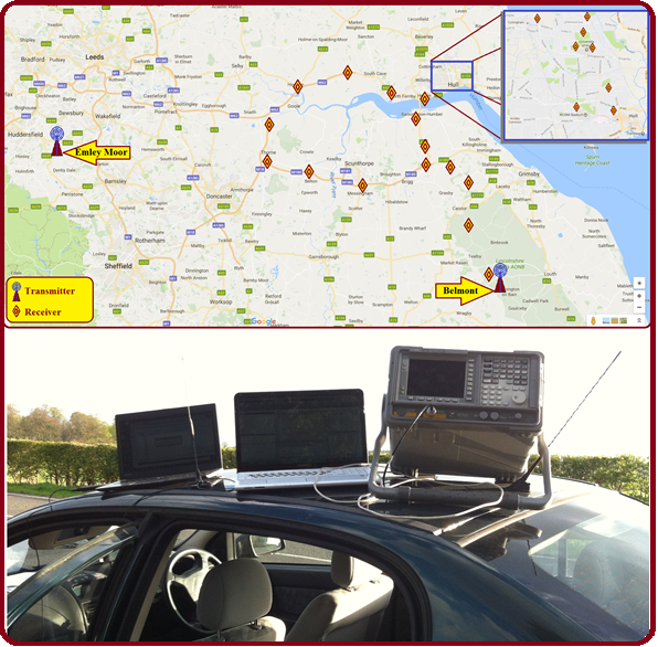Figure 3. Measurement equipment and geographical location in Hull and surrounding areas.

The measurement equipment used includes an omnidirectional antenna (covering the frequency range 174 to 230 MHz (VHF) and 470 to 790 MHz (UHF) with gain of 3.5 dBi) and spectrum analyser (Agilent E4407B, frequency range 9 kHz to 26.5 GHz) which was connected with a laptop computer by using a general purpose interface bus. A Matlab program on the laptop received raw data and stored them in (bin) files. In addition, the measurement locations were determined by using a mobile GPS application.

6.       ANALYSIS ofModels’Performance

6.1.  Propagation Path Loss Analysis

The main criterion for model assessment is path loss. A simulation program was implemented in Matlab, using channel 33 to conduct the comparison between the three propagation models and the measured results. In order to compare the real measurements with different propagation models, the path loss should be extracted from the real measurements by using the following equation in each location [9].

Where TX denotes the transmitted power, transmitting antenna gain is represented as TX_gain, PL is the path loss, receiving antenna gain is denoted as PR_gain and RP is the received power, dBm.

To evaluate the propagation models against real measurements, several parameters might be used to identify the most accurate propagation model. The error between predicted and measured path loss values was calculated by Equation 8 and the average error calculated by Equation 9.

In which e_i is denoted as the difference between the calculated path loss E_Pi and measured path loss M_pi derived from measured received power in each location.

Equations 8 and 9 are then used to calculate the standard deviation, Equation 10, whilst Root Mean Square Error (RMSE) is calculated by Equation 11, which also depends on the average error calculated in Equation 9.

To remove the influence of dispersion from the overall error, a significant metric can be derived from RMSE by subtracting the standard deviation of the absolute value of the error to obtain the Spread Corrected Root Mean Square Error (SCRMSE), as illustrated in Equations 12 and 13:

6.2.  Diffraction Factor Based on Terrain Profile Database

A common phenomenon that exemplifies the wave property of EM waves and light is diffraction, which is the bending of EM waves around obstacles. Diffraction is considered as a non-line of sight (NLOS) propagation mechanism which may occur when the propagation path is obscured by a barrier such as a mountain or hill or man-made obstacles including buildings. Diffraction can be the  cause of significant signal weakness at the reception site, due to the presence of some of the aforementioned barriers between the transmitter and receiver. There are two types of diffraction. “Shadow diffraction”, occurs when the received signal is blocked by obstacles and the received field strength will be decreased when the reception site is within the shadowed area. The second case, which occurs if the impediment is underneath the LOS, is called “lit diffraction,” and commonly leads to multi-path interference. Shadow diffraction is the one of the main reasons for increased the path-loss. One of the common diffraction models is the single knife edge model, explained by Huygens’s Principle, which states that when an electromagnetic wave is obstructed by a natural or man-made obstruction, the obstruction acts as a secondary source for creating a new wavefront which then propagates into the geometric shadow region of the obstruction [10].

6.3.  Terrain Profile-based Diffraction Model

One of the main effects of the terrain profile is to cause diffraction or bending of EM waves around obstacles such as mountains, hills or man-made structures which obscure the direct path.

In previous work [11], we considered terrain resolutions of 1 and 30 arcsec and determined that each of them had advantages and disadvantages in terms of accuracy and calculation time.

In this work, we attempt to improve these results by investigating a third resolution value between 1 and 30 arcsec to improve the compromise between accuracy and implementation time. For example, whilst calculating diffraction using the three different resolutions and investigating its effect on the received signal, we noticed that in the location approximately 38 km along the path shown in Figure 4, in the 30 arcsec resolution the elevation value is 100 m, whilst when using 3 arcsec and 1 arcsec resolution, the elevation values are approximately 86 and 83 m respectively.

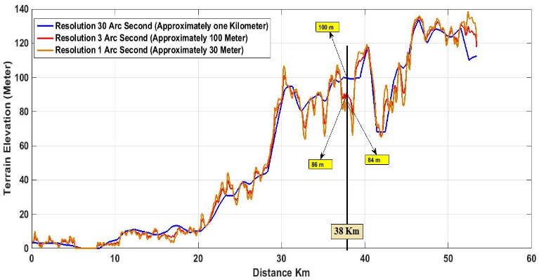Figure 4. Terrain elevation data for the path from University of Hull to Belmont TV Transmitter in different resolutions

Using 30 arcsec resolution takes a short time for the implementation process but has less accuracy. When using 1 arcsec, we have good accuracy but a long time for the implementation process. However, using 3 arcsec resolution produces the best results in terms of the compromise between accuracy and implementation time.

7.       Comparison and Results

The measurement study covered the area around the city of Hull, which was represented to measure the UHF TV band from 470 to 790 MHz with consideration of all radio and TV stations that feed the whole Hull area. Most of the channels transmitted into the area originate from the Belmont and Emley Moor transmitters (see Figure 3). The results of comparison of predicted path loss with measurements for two cases (excluding and including terrain modelling) are presented by using the previously defined criteria average error, standard deviation, RMSE and SCRMSE. Figure 5 shows our Graphical User Interface (GUI) of expected results including path loss curves for each propagation model and a table of calculated parameters.

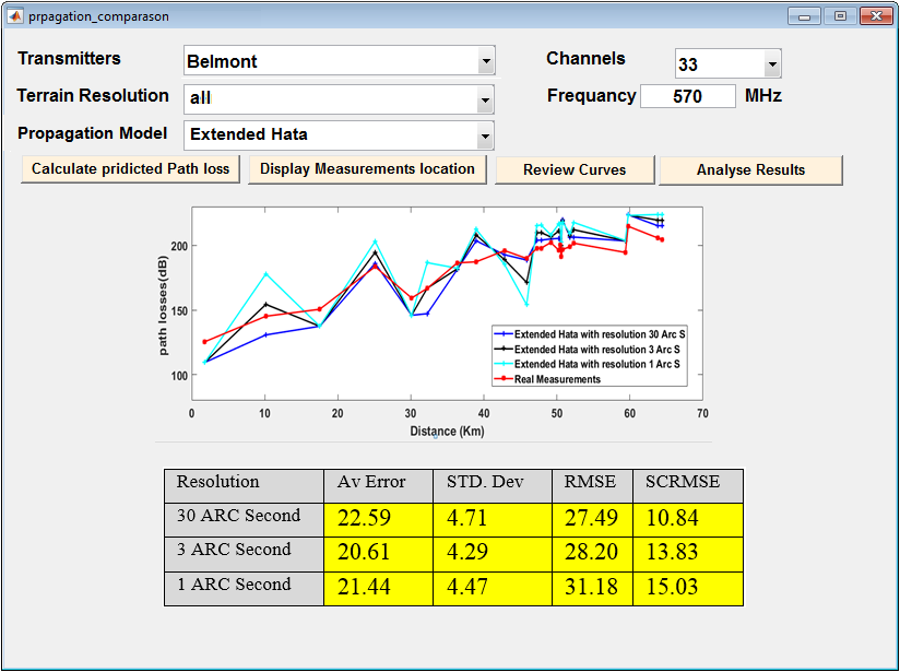Figure 5. GUI showing propagation model comparison in the selected measurement locations

This analysis may be undertaken for all selected measurement points, by flexible selection of the transmitter  name, terrain resolution, propagation model and transmitted channel. Results corresponding to all measurement locations and comparison of the three propagation models with real measurements along with parameter analysis, are discussed and classified in the following sections.

7.1.  Influence of Terrain Resolution on Results from the Extended Hata Model.

In this and in the following sections, terrain profile databases with various spatial resolutions and equivalent single knife edge diffraction have been used to calculate the diffraction factors and then evaluate their impact on the performance of the propagation models. The results in Table 2 indicate that 30 arcsec resolution used with the Extended Hata model can be considered the best fit to the measured data with low error when applying the diffraction factor at different terrain resolutions. It can be clearly seen in Figure 6 that the behavior of path loss was influenced by diffraction, when compared with the path loss derived from measured data.

Thus, the propagation behaviour has been affected  in most measurement locations when applying the terrain variation with 30 arcsec resolution. The impact of the propagation model is obvious after the third measurement point, where the first three points might be situated within the line of sight and the 1 km resolution results might have missed terrain features situated along the path which might cause destructive or constructive diffraction. Thus, using 1 km resolution might not give accurate results. Also when using 1 arcsec resolution, the terrain variation becomes worse in this model, which additionally requires a significantly longer processing time. However, the 3 arcsec resolution gives only slightly different results and does not need a long time for calculation of terrain profile.

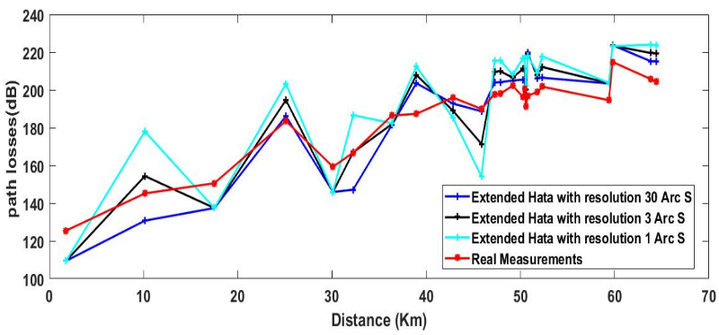Figure 6. Impact of terrain resolution on results from the Extended Hata model

In Table 2 we can observe how the error statistics have been impacted by the diffraction factor and how the SCRMSE value are decreased in the selected terrain resolution. The results indicate that the 30 arcsec and extended Hata model has the best results of the SCRMSE, at 10.84 dB. On the other hand, the 3 arcsec result is seen to have less error compared with 1 arcsec by about 1.2 dB.

Resolution, arcsec	Av Error, dB	STD. Dev, dB	RMSE, dB	SCRMSE, dB
30	23.34	4.87	23.52	11.07
3	21.43	4.47	22.82	9.95
1	22.23	4.64	25.02	9.81

Table 2: Fitted Extended Hata model in different terrain resolution

Resolution, arcsec	Av Error, dB	STD. Dev, dB	RMSE, dB	SCRMSE, dB
30	24.46	5.10	30.70	12.48
3	22.44	4.68	31.50	15.60
1	22.99	4.79	34.38	16.94

7.2.   Influence of Terrain Resolution on Egli Model Results.

Due to the nature of the terrain profile near the transmitter sites, which includes rough terrain and hills, the use of 1 arcsec and 3 arcsec resolutions will clearly affect the Egli propagation predictions, as illustrated in Figure 7. Here it may be seen clearly that there are large changes in the path loss at the distance of 48 km and that at other locations such around 52 km there is less variation where the receiver might be in line of sight of the transmitter.

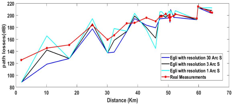Figure 7. Impact of terrain resolution on the Egli model results

The error of the SCRMSE for the both 1 arcsec and 3 arcsec are slightly different by about 0.14 dB as can be seen in Table 3, whereas the SCRMSE values for 30 arcsec resolution have increased by 1.12 dB.

Resolution, arcsec	Av. Error, dB	STD. Dev, dB	RMSE, dB	SCRMSE, dB
30	22.59	4.71	27.49	10.84
3	20.61	4.29	28.20	13.83
1	21.44	4.47	31.18	15.03

Table 3: Fitted Egli model in different terrain Resolutions

7.3.  Influence of Terrain Resolution on Davidson Model Results.

The Davidson model is clearly affected by terrain resolution in a similar manner to the Extended-Hata model at all selected resolution values, as shown in Figure 8.

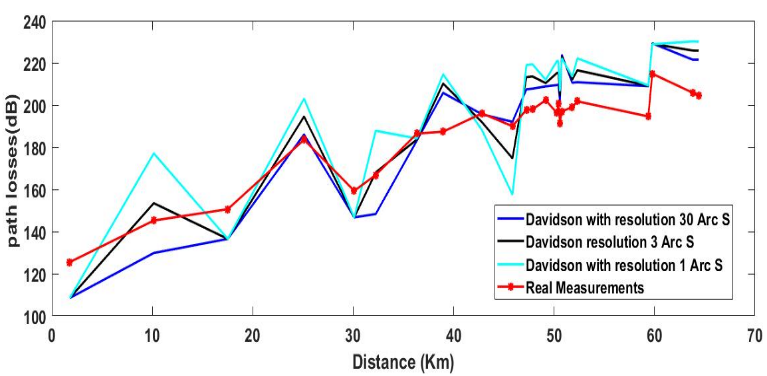Figure 8. Impact of different terrain resolution on the Davidson model

It can be observed in the statistics of Table 4 that the SCRMSE is increased while the resolution value is decreased as Table 2 of the Extended-Hata behavior.

Table 4: Fitted Davidson model in different terrain Resolutions

According to the advantage and disadvantage of both previous results in terms of accuracy and processing time, we observed that 30 arcsec has short time and less accuracy, while 1 arcsec has high accuracy and long processing time. Therefore, the 3 arcsec resolution in the Egli model gives the best result when taking these chosen criteria into account when comparing SCRMSE results between different terrain resolutions.

8.       Design of Flexible System for Creating TVWS Database by Using Different Propagation Models

 Based on the previous results, which indicate that the Egli model is the best among the models that have been chosen for comparison with the real measurements, a flexible system has been built that performs many functions related to propagation modelling and calculation of signal strength in each pixel. Among these tasks, it is possible to determine any geographic area based on latitude and longitude between two concentric points. In addition, it can be determined that the size of each pixel will affect the implementation time and propagation accuracy. Also, the system can perform three major operations at the same time to create a database for a selected geographic region that can be easily used when connected to the white space devices (WSD). In this work, for illustration, we considered only six transmitters, but more can be added using the “Add Transmitter Detail” button, as shown in Figure 9.

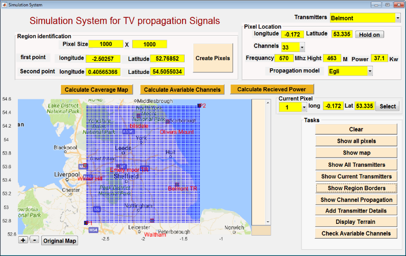Figure 9. Display of all pixels in the selected region in the flexible simulation system for creating TVWS database.

8.1.  Methodology for Calculation of Received Power

The second methodology to be implemented after creating the pixel file is to calculate the receiver power in each pixel in the frequency range 470 to 790 MHz, by considering the selected transmitters. The processing time depends on the number of pixels, propagation model and also the terrain resolution level. The process will be conducted only once to create a complete database of all the predicted TV signals in each pixel, as shown in Figure 10, which can be used for the next stages.

8.2.  Methodology for Calculation of Available Channels

The main goal of the system is to calculate available channels with high accuracy and then store all available channels of each pixel in the database, in a way which makes it easy to retrieve the data from WSDs. All of the transmitter information, such as height, channels and transmitted power, is stored previously in the database. The process takes into account all channels of the selected transmitters that might be received in a specific pixel, considering the weak signals as well.

8.3.  Methodology for Calculation of Coverage Map

This methodology must be used to translate the database that has been stored to show as a visual map of different levels of signal strength in the selected region for each transmitter, which are then stored in different files in the database as shown in Figure 11.

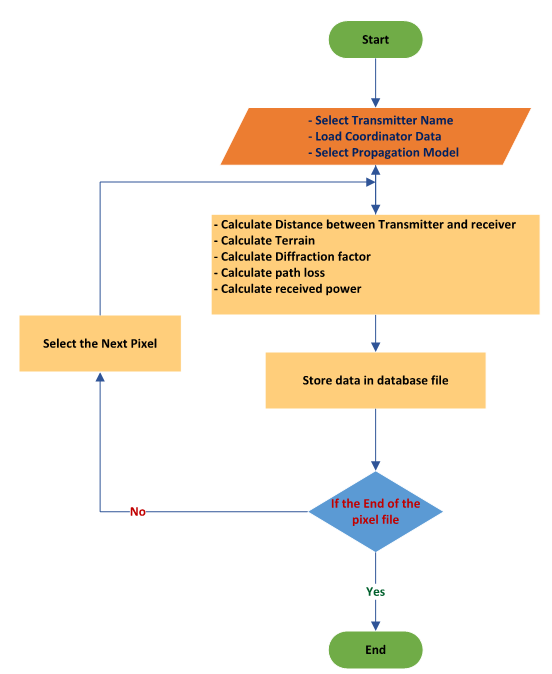Figure 10. Algorithm of the received power calculation

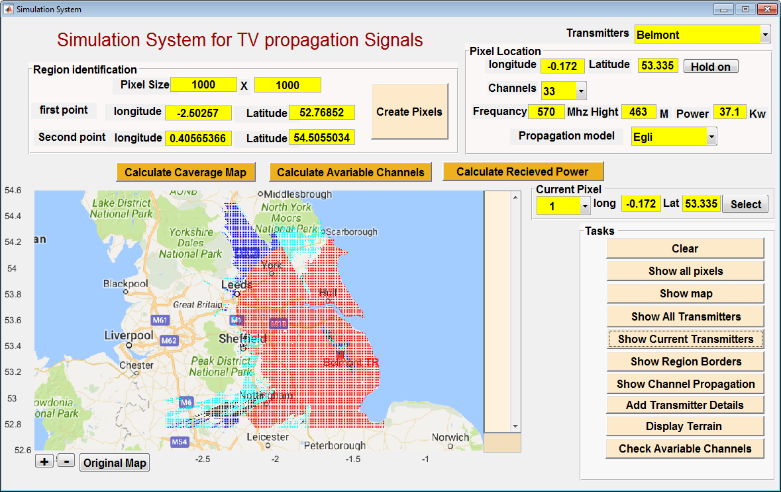Figure.11 Display of the propagation signals for channel 33 using Egli model.

9.       Conclusion

In this paper, TV signal strengths are calculated using various propagation models and then compared with real measurements that have been conducted in various locations. Using a single knife edge model to calculate the diffraction factor with consideration of terrain profile data at different resolutions, we investigate and prove how the terrain data resolution impacts the accuracy and implementation time of the propagation models. We have improved and extended results that have been published in our conference paper in 2016 [11]. RMSE and SCRMSE are the main criteria taken into account to assess the propagation models in different terrain resolutions. The results show that the Egli model still gives the best results when account is taken of the terrain profile data at a resolution of 3 arcsec (100m), providing SCRMSE of 0.14 dB, with shorter computation time and similar accuracy as compared with 1 arcsec. On the other hand, RMSE and SCRMSE values of the extended Hata and Davidson models are still increasing and have poor performance when terrain data resolution is decreased. Therefore, 3 arcsec is considered the best resolution that can be used to calculate diffraction factor. The results also show that the Egli model is the best model giving a consistently good fit to measured data among other selected models and, with appropriate terrain data, will provide useful input to a system for facilitation of the cognitive radio decision process. In addition, the main benefits for designing the flexible system is to create a TVWS database for a specific area, by selecting the optimum pixel size, adding appropriate transmitter information and choosing a suitable propagation model. In future work, the system will be developed to use additional propagation models at various terrain data resolutions, providing a clear understanding of the differing results between propagation models taking into account the terrain resolution.

Acknowledgment

The lead author is grateful to his supervisor for his unlimited supporting to develop this study, by providing the suitable solutions and suggestions.

Conflict of Interest

The authors declare no conflict of interest.

1. Gurney, D., Buchwald, G., Ecklund, L., Kuffner, S.L. and Grosspietsch, J., 2008, October. Geolocation database techniques for incumbent protection in the TV white space. In New Frontiers in Dynamic Spectrum Access Networks, 2008. DySPAN 2008. 3rd IEEE Symposium on (pp. 1-9). IEEE.
2. National Imagery and Mapping Agency, “Digital Terrain Elevation Data,“ 30 May, 1990. ’www.globalsecurity.org/ intell/systems/dted.htm.
3. Nekovee, M., 2009, October. A survey of cognitive radio access to TV white spaces. In 2009 International Conference on Ultra Modern Telecommunications & Workshops (pp. 1-8). IEEE.
4. Iskander, M.F. and Yun, Z., 2002. Propagation prediction models for wireless communication systems. Microwave Theory and Techniques, IEEE Transactions on, 50(3), pp.662-673.
5. P. Pardeep, P. Kumar and B. S. Rana, “Performance evaluation of different path loss models for broadcasting applications,” American Journal of Engineering Research (AJER) , 3(4), pp.335-342, 2014.
6. K. Stylianos, P. I. Lazaridis, Z. D. Zaharis, A. Bizopoulos, S. Zettas, and J. Cosmas, “Comparison of Longley-Rice, ITU-R P. 1546 and Hata-Davidson propagation models for DVB-T coverage prediction, ” In BMSB, pp. 1-4, 2014.
7. J. J. Egli, “Radio propagation above 40 MC over irregular terrain. Proceedings of the IRE, ” , 45(10), pp.1383-1391,1957.
8. M. Hope, A. B. Bagula, M. Zennaro, and G. Lusilao-Zodi, “On the impact of propagation models on TV white spaces measurements in Africa,“ International Conference on. IEEE, pp.148-154, May 2015.
9. P. Prajesh, and R. K. Singh, “Investigation of outdoor path loss models for wireless communication in Bhuj,“ International Journal of Electronics and Communication Engineering & Technology (IJECET), Volume 3, Issue 2, pp. 171-178, September 2012.
10. J. You-Cheol, “Diffraction analysis and tactical applications of signal propagation over rough Terrain,” Air Force INST of Tech Wright-Patterson AFB OH School of Engineering, no. 97J-01, Dec 1997.
11. A. M. Fanan, N. G. Riley, M. Mehdawi, and M. Ammar, 2016, November. Comparison of propagation models with real measurement around Hull, UK. In Telecommunications Forum (TELFOR), 2016 24th (pp. 1-4). IEEE.

(Click to view)

(Click to view)