1. Introduction

The concept of controllability has been widely developed since the sixties [1,2]. Later, the notion of regional controllability was introduced by El Jai [3,4], and interesting results have been obtained, in particular, the possibility to control a state only on a subregion ω of Ω. These results have been extended to the case where ω is a part of the boundary ∂Ω of the evolution domain Ω [5,6]. Then the concept of regional gradient controllability and regional enlarged controllability were introduced and developed for linear and semilinear systems [7–11]. Here instead of steering the system to a desired gradient, we are interested in steering its gradient between two prescribed functions given only on a boundary subregion Γ ⊂ ∂Ω of system evolution domain .

Many reasons are motivating this problem: first, the mathematical models are obtained from measurements or from approximation techniques and they are very often affected by perturbations. And the solution of such system is approximately known. Second, in many real problems the target required to be between two bounds. Moreover, there are many applications of gradient modeling. For example, controlling the concentration regulation of a substrate at the upper bottom of a bioreactor between two levels (see Figure1).

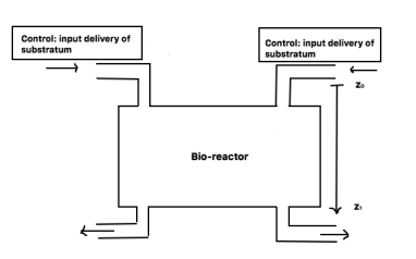Figure 1: Regulation of the concentration flux of the substratum at the upper bottom of the bio-reactor

Motivated by the arguments above, in this paper, our goal is to study the regional boundary enlarged controllability of the gradient. For that we consider a semilinear system of parabolic equations where the control is exerted in an intern subregion ω of the system evolution domain Ω.

Thus, let Ω be an open bounded set of Rⁿ(n ≥ 1) with regular boundary ∂Ω. We consider the Banach spaces L²(Ω) and H) with their corresponding norms. For a given T > 0, we denote Q_T = Ω×]0,T [, Σ = ∂Ω×]0,T [ and we consider the following problem

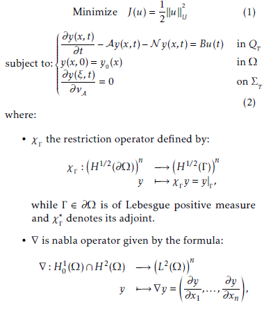• γ : L²(Ω)^{n →} H^1/2(∂Ω)ⁿ is the extension of trace operator of order zero which is linear, continuous and surjective,
• y_u (T ) is the mild solution of (2) at the time T

) [12]), and u is a the control function in the control space U = L²(0,T ;R^m) (where m is the number of actuators),

• A is linear, second order operator with dense domain such that the coefficients do not depend on t and generates a C₀-semigroup (S(t⁾⁾_t≥₀ on L²(Ω) which we consider compact,
• N : L²(0,T ;L²(Ω)) → L²(Ω) is a non linear k-

Lipschitz operator [13],

• B ∈ L _R^m,L²(Ω) and y₀ is the initial datum in L²(Ω).

The problem (1-2) is well-posed and has a unique solution.

The remainder contents of this paper are structured as follows. Some preliminary results are introduced in the next section. In section 3 we give the definitions of the gradient enlarged controllability on the boundary. Two approaches steering the system (2) from the initial gradient vector to a target gradient function between two bounds with minimum energy control is presented in section 4.

2. Preliminary results

In this section, we introduce some preliminary results to be used there after.

Let D be an open subset of L²(Ω), we consider the system in (2), where y₀ ∈ D and y : [0,T ] → D. A continuous function u : [0,T ] → D is said to be a classical solution of (2) if u(0) = y₀(x), u is differentiable on [0,T ]. and u(t) ∈ D for t ∈ [0,T ] and y satisfies (2) on [0,T ].

It is well known that if y is a classical solution of (2), then it satisfies the following:

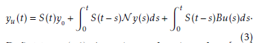Definition 1 (14) A continuous function y from [0,T ] into D is called a mild solution of (2) if y satisfies the integral equation (3) on [0,T ].

Let Γ ⊆ ∂Ω a part of the boundary with y(x,t) satisfies

(3), then the regional enlarged controllability on the boundary problem is concerned whether there exists a control u to steer the system (2) from the initial gradient vector ∇y₀ to a gradient vector between two

n functions in H.

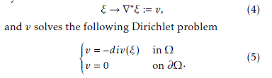
By [15], the adjoint of the gradient operator on a connected, open bounded subset Ω with a Lipschitz continuous boundary ∂Ω is the minus of the divergence operator. Then ∇^∗ : (L²(Ω))ⁿ → H⁻¹(Ω) is given by

We recall the following definitions

Definition 2 (16) The system (2) is exactly (resp.

weakly) gradient controllable on Γ if for every desired n

gradient g_d(resp. for every  > 0), there exists a control u ∈ U such that χ_Γ γ ∇y_u(T ) = g_d (resp.

k

We recall that an actuator is conventionally defined by a couple (D,f ), where D is a nonempty closed part of Ω, and it represents the geometric support of the actuator. And f ∈ L²(D) defines the spatial distribution of the action on the support D. For more details about the notion of actuators we refer the readers to [3,17].

We need also to recall this important result:

Theorem 1 Let (X,(^·, ^·)_X , ^{k · k}_X ), (Y,(^·, ^·)_Y , ^{k · k}_Y ) be two Hilbert spaces and let A ⊆ X, B ⊆ Y be non-empty, closed, convex subsets. Assume that a real functional L : A × B → _R satisfies the following conditions

∀µ ∈ B, v → L(v,µ) is convex and lower semicontinuous;

∀v ∈ A, µ → L(v,µ), is concave and upper semicontinuous.

Moreover,

• is bounded or lim L(v,µ₀) = +∞ ∀µ₀ ∈ B kv k_X → ∞

v ^∈ A

• is bounded or−∞

kµk_Y µ ^∈ B

Then, the functional L has at least one saddle point.

Demonstration: For the proof of this theorem see [18].

3. Gradient enlarged controllability on the boundary

In this section, we give the definition of the concept of the gradient enlarged controllability on the boundary. To do so, we need to introduce the closed sub-vectorial space G of H₀¹(Ω). Hence, we have the following definition:

Definition 3 Given T > 0. We say that there is gradient enlarged controllability on Γ, if, for every y₀ (in a suitable functional space), we can find a control u such that χΓ γ ∇yu (T ) ∈ G

Remark 1 • This notion depends of course on the choice of the functional space G.

• If G = {0}, we retrieve the classical notion of the exact controllability.
• if G is the space skimmed by y_u (T ), the notion is empty.

For the particular case, we will study the boundary gradient enlarged controllability in [a_i(·),b_i(·)] ∀i ∈ {1,…,n}. For that let’s consider (a(·))_i and (b(·))_i be two given functions in H^1/2(Γ)ⁿ such that (a(·))_i ≤ (b(·))_i for i = 1,…,n a.e on Γ, and we set:

Θ = [a (·),b (·)] =

ⁿ(y₁,…,y_n)                                      (·) ≤ y_i(·) ≤ b_i(·)        a.e on Γ^o

                                    for all i ∈   {1,…,n}

So the definition of the boundary gradient enlarged controllability in Θ is the following:

Definition 4 We say that (2) is Θ-gradient controllable on Γ at time T if there exist a command u ∈ U such that: χΓ γ ∇yu (T ) ∈ Θ ·

Let us define the following operators:

• The Duhamel operator H from U to H such that for u ∈ U:

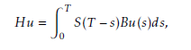• and the operator G_Θ given by:

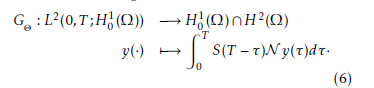Finally, the solution of the system (2) at the time T could be written as follow: y_u (T ) = S(T )y₀ +G_Θy +Hu · And we have the following proposition:

Proposition 1 We say that system (2) is Θ-gradient controllable on Γ at time T if and only if:

Imχ_Γ γ ^∇G_Θ +Imχ

Demonstration: We suppose that the system (2) is Θgradient controllable on Γ at time T which is equivalent to write: χ_Γ γ ∇y_u (T ) ∈ Θ. Hence we can write:

Hu= χ_Γ γ ^∇S(T )y₀ +χ_Γ γ ^∇G_Θy +χ_Γ γ ^∇Hu.

And we have ∇S(T )y₀ = 0, furthermore, let’s denote by:             z₁ = χ_Γ γ ∇G_Θy, z₂ = χ_Γ γ ∇Hu and z =

             χ_Γ γ ∇y_u (T ).           Which leads to:    z₁ ∈ Im χ_Γ γ ∇G_Θ

 and z₂ ∈ Im.               Thus, z ∈ Im

Im χ_Γ γ ∇H and z ∈ Θ which gives:

Imχ_Γ γ ∇G_Θ +Imχ

Conversely, we suppose that the following expression is verified:

Imχ_Γ γ ∇G_Θ +Imχ,

then,       there      exists     z         ∈ Θ such         that     z      ∈

Imχ_Γ γ ∇G_Θ +Imχ_Γ γ ∇H . So z = z₁ + z₂ where z₁ = χ_Γ γ ∇G_Θy with y ∈ L²(0,T ;H )) and ∃ u ∈ U such that z₂ = χ_Γ γ ∇Hu. Then z = χ_Γ γ ∇G_Θy +χ_Γ γ ∇Hu. While χ_Γ γ ∇S(T )y₀ = 0, one can write: z = χ_Γ γ ^∇S(T )y₀ +χ_Γ γ ^∇G_Θy +χ_Γ γ ^∇Hu

Hence, z = χ_Γ γ ∇y_u (T ) ∈ Θ, and we prove the equivalence.

Remark 2 1. The above definition means that we are interested in the transfer of the system (2) to an unknown state just in Θ.

2. If Θ = {0} or a_i(·) = b_i(·) ∀i ∈ {0,1} we retrieve the regional exact controllability. So, for a_i(·) , b_i(·) the Θ-gradient controllability on Γ constitutes an extension of the regional controllability.

We can also characterize the enlarged controllability by using the notion of strategic actuators. And we can say:

Definition 5 The actuator (D,f ) is said to be Θ-strategic on Γ if the excited system is Θ-gradient controllable on Γ.

4. Computation of the control

In order to compute the control subject to our problem

(1-2), we will use two approaches. The first one relies on the subdifferential techniques and convex analysis and the second one on the Lagrangian multiplier approach.

4.1. Subdifferential approach

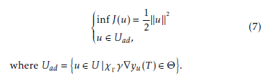
In this sub-section we are using the subdifferential techniques to compute the control steering the system from an initial gradient state to a final one between two functions on the boundary [19,20]. For that, we consider the optimization problem in (1).

• Let f be a nontrivial, lower semi-continuous, proper and convex function from a Hilbert space W to R_e=] − ∞,+∞[. We denote F (W) the set of the functions f and k · k is the Hilbert norm of W.
• For f ∈ F (W), the polar function f ^∗ of f is given by f ∗(v∗) = sup {hv∗,v i − f (v)} ∀v∗ ∈ W v∈dom(f )

where dom(f ) = {v ∈ W | f (v) < +∞}.

• For v₀ ∈ dom(f ), the set:

∂f (v0) = nv∗ ∈ W | f (v) ≥ f (v0)+ hv∗,v − v0 i ∀v ∈ Wo denotes the subdifferential of f at v₀, then we

∗

have v₁ ∈ ∂f (v ) if and only if f (v∗)+f ∗(v1) = hv∗,v1 i

With all these notations, the problem (7) is equivalent to:

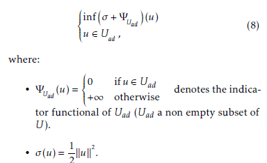tor functional of U_ad (U_ad a non empty subset of U).

2

• σ(u) =ku k .

Hence the solution of (8) is characterized by the following result.

Theorem 2 u^∗ is a solution of (7) if and only of if the system (2) is Θ-gradient controllable on Γ and:

                   u∗ ∈ Uad           and ΨU∗ad (−u∗) = −ku∗ k2 ·               (9)

Demonstration: The system (2) is Θ-gradient controllable on Γ, then U_ad , ∅. Using Fermat’s rule, we have u^∗ is a minimum of (7) if and only if 0 ∈ ∂ σ +Ψ_Uad (u ).

We prove that U_ad is convex, for that we consider u and v two elements of U_ad. So χ_Γ γ ∇y_u (T ) ∈ Θ and χ_Γ γ ∇^y_tu+(1−_t)v (T ) ∈ Θ for t ∈ [0,1] which prove the convexity.

And we have σ ∈  F (U) and since U_ad is closed, convex and non empty, then Ψ_Uad ∈             F (U)

Moreover, domσ ∩ domΨ_U , ∅ because the system (2)

ad is Θ-gradient controllable on Γ.

Furthermore,_Uad (u ) = ∂σ(u ) + ∂Ψ_Uad (u ) (σ ∗ is continuous). It follows that u is a solution of (7) if and only if 0 ∈ ∂σ(u^∗)+∂^Ψ_Uad (u^∗).

Besides we have σ is Frechet-Differentiable, hence ∂σ(u^∗) = {u^∗ }. Furthermore, u^∗ is the solution of (7) if and only if −u^∗ ∈ ∂Ψ_Uad (u^∗) which is equivalent to Ψ_Uad (u^∗) + Ψ_U^∗_ad (−u^∗) = −ku^{∗ k2}. And which gives u∗ ∈ Uad and ΨU∗ad (−u∗) = −ku∗ k2.

4.2. Lagrangian approach

We consider the problem (1) when the system (2) is excited by one actuator (D,f ). The following result gives a useful characterization of the solution of the problem.

Theorem 3 If the system (2) is Θ-gradient controllable on Γ then the solution of (1-2) is given by:

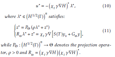while P→ Θ denotes the projection operator, ρ > 0 and RH.

Demonstration: If the system (2) is Θ-gradient controllable on Γ then U_ad , ∅ and the problem (1-2) has a unique solution.

The minimization problem (1) is equivalent to the following saddle point problem:

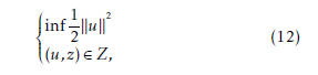where Z = (u,z) ∈ U_ad × Θ | χ_Γ γ ∇y_u (T ) − z = 0 .

To study this constraints, we will use a Lagrangian functional and steer the problem (12) to a saddle point problem.

We associate to the problem (12) the Lagrangian functional defined by:

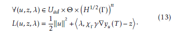We prove that L admits a saddle point: The set U_ad × Θ is non empty, closed and convex. The functional L satisfies these conditions:

• (u,z) 7→ L(u,z,λ) is convex and lower semin continuous for all.
• λ 7→ L(u,z,λ) is concave and upper semi-continuous for all (u,z) ∈ U_ad × Θ.

Moreover, there existssuch that:

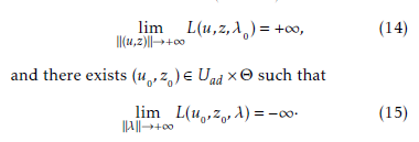kλk→+∞

Then, the functional L admits a saddle point. For more details we refer to [21]. We prove then that u^∗ is a solution of (1) and it is the minimum one:

Let (u^∗,z^∗,λ^∗) be a saddle point of L. Hence, we have:

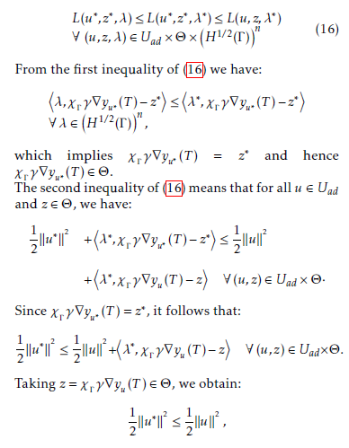
which implies that u^∗ is of minimum energy. . (u^∗,z^∗) is an optimal solution of (12), then there n exists a Lagrange multipliersuch that the following optimality conditions hold: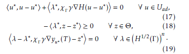

(19) For more details about the saddle point and its theory, we refer to [22–24]. From (17) we deduce (10). which is equivalent to the second equation of (11).

5. Conclusion

This paper is concerned with the regional gradient controllability, which is motivated by many real applications where the objective is to explore the minimum energy control to steer the system under consideration from the initial gradient vector ∇y₀ to any gradient vector in an interested subregion of the whole domain. The presented results here can provide some insight into the control theory analysis of such systems. They can also be extended to complex fractional order distributed parameter systems and various open questions are still under consideration.

6. Funds

The work has been carried out with a grant from Hassan II Academy of Sciences and Technology.

1. F. Curtain, H. Zwart, An Introduction to Infinite Dimensional Linear Systems Theory, Texts in Applied Mathematics, 21, Springer, New York, 1995.
2. F. Curtain, A. J. Pritchard, Infinite Dimensional Linear Systems Theory, Springer Lecture Notes in Control and Informations, Science, Springer, New York, 1978.
3. El Jai, A. J. Pritchard, Sensors and Actuators in the Analysis of Distributed Systems, Wiley, New York, 1988.
4. El Jai, M. C. Simon, E. Zerrik, A. J. Pritchard, ”Regional controllability of distributed parameter systems.”, International Journal of Control, 62(6), 1351-1365, 1995.
5. Zerrik, R. Larhrissi, ”Regional target control of the wave equation.”, Int. J. Syst. Sci., 32, 105-110, 2001.
6. Zerrik, R. Larhrissi, ”Regional Boundary Controllability of Hyperbolic Systems. Numerical Approach.”, Journal of Dynamical and Control Systems, 8, 293-311, 2002.
7. Zerrik, F. Ghafrani, ”Minimum energy control subject to output constraints numerical approach.”, IEE Proc.-Control Theory Appl., 149(1), 105-110, 2002.
8. Boutoulout, H. Bourray, F. Z. El Alaoui, L. Ezzahri, ”Constrained Controllability for Distributed Hyperbolic Systems.”, Math. Sci. Lett., 3(3), 207-214, 2014.
9. Karite, A. Boutoulout, ”Regional constrained controllability for parabolic semilinear systems.”, International Journal of Pure and Applied Mathematics, 113(1), 113-129, 2017.
10. L. Lions, E. Magenes, Problmes aux limites non homognes et applications, Dunod, 1, 1968.
11. Zeidler, Applied functional analysis : Applications to mathematical physics, Springer-Verlag, New York, 1995.
12. B. Agase, V. Rchavendre, ”Existence of mild solutions of semilinear differential equations in Banach spaces.”, Indian J. pure appl. Math., 21(9), 813-821, 1990.
13. Kurula, H. Zwart, ”The Duality Between the Gradient and Divergence Operators on Bounded Lipschitz Domains.”, Department of Applied Mathematics, University of Twente, October 2012.
14. Kamal, A. Boutoulout, S. A. Ould Beinane, ”Regional Gradient Controllability of Semi-Linear Parabolic Systems.”, International Review of Automatic Control, 6(5), 2013.
15. Zerrik, A. El Jai, A. Boutoulout, ”Actuators and regional boundary controllability of parabolic system.”, Int. J. Syst. Sci. 31(1), 73-82, 2000.
16. P. Aubin, S. Wilson, Optima and Equilibria: An Introduction to Nonlinear Analysis, Springer-Verlag Berlin Heidelberg, 2002.
17. Kusraev, S. S. Kutateladze, Subdifferentials: Theory and Applications, Springer Netherlands, 1995.
18. Matei, ”Weak solvability via Lagrange multipliers for two frictional contact models.”, Annals of the university of Bucharest (mathematical series), 4, (LXII), 179-191, 2013.
19. Brezzi, M. Fortin, Mixed and Hybrid Finite Element Methods, Springer-Verlag, New York, 1991.
20. Fortin, R. Glowinski, Augmented Lagrangian Methods: Applications to the numerical solution of boundary-value problems, North-Holland, 15, 1983.
21. T. Rockafellar, ”Lagrange multipliers and optimality”, SIAM Review, 35(2), 183-238, 1993.

(Click to view)

(Click to view)