1 Introduction

Low-density parity check (LDPC) codes are a class of linear block codes, which were first, introduced by gallager in 1963 [1]. As soon as they were re-invented in 1996 by mackay [2], LDPC codes have received a lot of attention because their error performance is very close to the shannon limit when decoded using iterative methods [3]. They have emerged as a viable option for forward error correction (FEC) systems and have been adopted by many advanced standards, such as 10 gigabit ethernet (10GBASET) [4], [5] and digital video broadcasting (DVB-S2) [6], [7]. In addition, the generations of WiFi and WiMAX are considering LDPC codes as part of their error correction systems [8], [9].

In the present paper, we propose the threshold multi split-row method for decoding irregular lowdensity parity-check (LDPC) codes [10], to have better performance in terms of bit error rate. We will apply the thresholding algorithm in [11] for multi split row of irregular LDPC codes[10]. The proposed split-row decoder [10],[11] splits the row processing into two or multiple nearly independent partitions. Each block is simultaneously processed using minimal information from an adjacent partition. The key idea of split-row is to reduce communication between row and column processors which has a major role in the interconnect complexity of existing LDPC decoding algorithms such as sum product (SPA) [3] and minsum (MS) [12]. This paper introduces threshold multi split-row decoding which significantly reduces wire interconnect complexity and considerably improves the error performance compared to non-threshold multisplit decoding [10]. The paper is organized as follows: Section II reviews the sum product and minsum, split-row and split-row threshold decoding algorithms. Threshold multi-split-row and its error performance result is presented in section III. Finally, the conclusion is in section IV.

2 Previous algorithms

2.1 Sum Product Decoding(SPD)

The SPD assumes a binary code word (x1;x2; :::;xN) transmitted using a binary phase-shift keying (BPSK) modulation. The sequence is transmitted over an additive white gaussian noise (AWGN) channel and the received symbol is (y1;y2; :::;yN). We define:

V(i) = fj : Hij = 1g as the set of variable nodes which participate in the check equation i. C(j) = fi : Hij = 1g as the set of check nodes which participate in the variable node j update.

Also

V(i) n j denote all variable nodes in V(i) except node j.

C_(j) \ i denote all check nodes in C_(j) except node i. Moreover, we define the following variables used in this paper.

λ_j : is defined as the information derived from the

log-likelihood ratio of received symbol y_j.

             λ_j = log(P (x_i = 0|y_j)/P (x_i = 1|y_j)) = (2y_j)/σ²                     (1)

where σ² is the noise variance. α_ij is the message from check node i to variable node j. This is the row processing output. β_ij is the message from variable node j to check node i. This is the column processing output.

The sum product algorithm decoding as described by mohsenin and Baas [13], can be summarized in the following four steps:

2.1.1        Initialization

For each i and j, initialize β_ij to the value of the loglikelihood ratio of the received symbol y_j, which is λ_j. During each iteration, αβ messages are computed and exchanged between variables and check nodes through the graph edges according to the following steps numbered 2-4.

2. Row processing or check node updateCompute α_ij messages using β messages coming from all other variable nodes connected to check node C_i,

excluding the β information from Vj:
Y αij =                  sign(βij0 ) × φ(Σj0 ∈V (i)\jφ(|βij0 |)) 0 j ∈V (i)\j where the non-linear function	(2)
φ(x) = −log(tanh(|x|/2))	(3)

The first product term in the equation that update the parameter, is called the parity (sign) update and the second product term is the reliability (magnitude) update.

3. Column processing or variable node updateCompute β_ij messages using channel information λ_j and incoming, messages α; from all other check nodes connected to variable node V_j, excluding check node

C_i.

                                   βij = λj +Σi0 ∈C(j)\iα(i0 j)                                             (4)

4. Syndrome check and early terminationWhen the column processing is finished, every bit in column j is updated by adding the channel information λ_j and α, messages from neighboring check nodes.

                                    zj = λj +Σi0 ∈C(j)α(i0 j)                                                (5)

From the updated vector, an estimated code vector

X_b= {_bx₁,_bx₂,…,_bx_N } is calculated by:

_i

If H ×_bx^t = 0 then X_b is a valid codeword and therefore the iterative process has converged and decoding stops. Otherwise, the decoding repeats from step 2 until a valid codeword is obtained or the number of iterations reaches a maximum number, which terminates the decoding process.

2.2       MinSum Decoding

The check node or row processing stage of SP decoding can be simplified by approximating the magnitude computation in Eq. 2 with a minimum function. The algorithm using this approximation is called minsum (MS):

Y

              αij =                  sign(βij0 ) × Minj0 ∈V (i)\j(|βij0 |)         (7)

0

j ^∈V (i)^\j

In MS decoding, the column operation is the same as in SP decoding. The error performance loss of MS decoding can be improved by scaling the check (α) values in Eq. 7 with a scale factor S ≤ 1 which normalizes the approximations [14], [15].

Y

        αij = S ×                  sign(βij0 ) × Minj0 ∈V (i)\j(|βij0 |)        (8)

0

j ^∈V (i)^\j

2.3    Split Row and Split Row Threshold Decoding

Recall that a standard message passing two-phase algorithm consists of a check node update followed by a variable node update as shown in Fig. 1 (a). The basic idea in split-row [10], [16] and split-row threshold [11], is to divide the check node processing into two or multiple nearly-independent partitions. Each check node processor, simultaneously, computes a new message while using minimal information from its adjacent partitions. Split-row is illustrated in Fig. 1 (b) showing how the check node processing is partitioned into two blocks. A single bit of information (Sign) for each check node processor must be sent between partitions to improve the error performance.

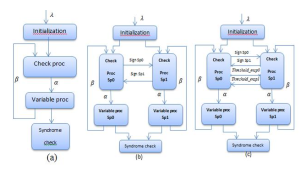Figure 1. Block diagram of (a) standard two-phase decoding (b) split-row (c) split-row threshold block diagram.

The loss error performance is 0.5-0.7 dB of split-row that is the major drawback, when compared to minsum normalized and SPA decoders. This performance degradation is dependent on the number of check node partitions. For minsum split-row each partition has no information of the minimum value of the other partition, and a Sign signal is sent to minimize the error due to incorrect sign information of the true check node output α.

The split-row threshold algorithm mitigates the error caused by incorrect magnitude by providing a signal, threshold en, which indicates whether a partition has a minimum less than a given threshold (T).This causes all check nodes to take the min of their own local minimum or T. Thus, any large deviations from the true minimum because of the partitioning are reduced, which then makes multi-split implementations feasible.

Figure 1 (c) shows the additional single bit signal (threshold en ) added to the original split-row architecture by the split-row threshold algorithm. This signal allows the split-row to remain essentially unchanged while adding some extra logic and minimal wiring to improve error significantly [11].

Therefore, the split-row architectures reduce the communication between check node and variable node processors, which is the major cause of the interconnect complexity found in existing LDPC decoder implementations.In addition, the area of each check node processor will be reduced. However, note that the variable node operation in the SPA, minsum, splitrow and split-row threshold algorithms are all identical. Thus, the logic of the variable node processor is left unchanged.

3 Threshold Mutli Split Row Decoding

3.1               Threshold Mutli Split Row Algorithm

In order to increase the parallelism and reduce the complexity of the decoder, the multi-split-row method divides the lines of the systematic submatrix Hs into Spn blocks called split-Spn. This approximation requires of the wire to correctly process the sign bits between the blocks. For the threshold multi split-row method, Each partition sends the status of its local minimum against a threshold to the next partition with a single wire, called T hreshold ensp.

The block diagram of threshold multi split-row decoding with Spn partitions, highlighting the sign and T hreshold ensp passing signals, is shown in Fig. 2. These are the only wires passing between the partitions [17]. In each partition, local minimums are generated and compared with a threshold T simultaneously. If the local minimum is smaller than T then the T hreshold ensp signal is asserted high. The magnitudes of the check node outputs are finally computed using local minimums and the T hreshold ensp signal from neighboring partitions.

0

If a local partition s minimums are larger than T , and at least one of the T hreshold ensp signals is high, then T is used to update its check node outputs. Otherwise, local minimums are used to update check node outputs.

in the threshold multi split-row algorithm, as shown in Eq. (10) and (11), the first and second Mins are compared with a predefined threshold, and a single-bit threshold-enable (T hreshold en out) global signal is sent to indicate the presence of a potential global minimum to other partitions.

3.1.1        Initialization

The first and second minimums are determined for each partition according to the following relationships:

Minj0 ∈V (i)\j(|βij0 |) = ( MinMin12ii;; ifif ;; jj ,= argminargmin((MinMin11ii))

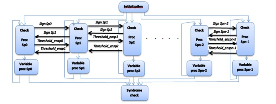Figure 2. Block diagram of threshold multi split row decoding with Spn partitions.

(9)

                                Min1_i = min_j∈V (i)(|^β_ij⁰ |)                        (10)

Min2i = minj00 ∈V (i)\argmin(min1i)(|βij00 |) (11) to execute the algorithm one needs the number of partitions and the threshold value T. Finds T hreshold ensp(i) out(i∓1) for the ith partition of a spn-decoder.

Algorithm 1 Threshold Multi Split-Row Algorithm

1-if Min1_i ≤ T and Min2_i ≤ T then

Threshold ensp(i) out(i ∓ 1) = 1

Minj0 ∈V(i)\j(|βij0 |) = ( MinMin21ii if jif j ,=argminargmin((MinMin11ii)) (12)

• if Min1_i ≤ T and Min2_i ≥ T then

Threshold ensp(i) out(i ∓ 1) = 1 Threshold ensp(i +1) == 1 or

Threshold ensp(i − 1) == 1 then

        Minj0 ∈V(i)\j(|βij0 |) = ( MinT if1i jif= argminj , argmin(Min(Min1i) 1i) (13)

else
( Min1 Minj0 ∈V(i)\j(|βij0 |) = Min2ii ifif end if	j , argmin(Min1i) j = argmin(Min1i)

• else if Min1_i ≥ T and (Threshold ensp(i +1) == 1 or

Threshold ensp(i − 1) == 1) then Threshold ensp(i) out(i ∓ 1) = 0

                                    Minj0 ∈V(i)\j(|βij0 |) = T                               (14)

• else

Threshold ensp(i) ou(i ∓ 1) = 0

_i if j , argmin(Min1_i)             (15) i if j = argmin(Min1i)

end if.

The kernel of the threshold multi split-row algorithm is given in Algorithm 1. As shown, four conditions will occur:

Condition 1: both Min1 and Min2 are less than threshold T. In this case these 2 parameters are used to calculate α messages according to Eq.(12). In addition, T hreshold ensp(i) out(i∓1), which represents the general threshold-enable signal of a partition with two neighbors, is asserted high indicating that the least minimum (Min1) in this partition is smaller than T.

Condition 2: only Min1 is less than T. As Condition 1 T hreshold ensp(i) out(i∓1)= 1. If at least one T hreshold ensp(i ∓ 1) signal from the nearest neighboring partitions is high, indicating that the local minimum in the other partition is less than T, then we use Min1 and T to calculate α messages according to Eq.(13). Otherwise, we use Eq.(12).

Condition 3: when the local Min1 is larger than T and at least one T hreshold ensp(i∓1) signal from the nearest neighboring partitions is high; thus, we only use T to compute all α messages for the partition using

Eq.(14).

Condition 4: when the local Min1 is larger than T and if the T hreshold ensp(i∓1) signals are all low; thus, we again use Eq.(12).

The variable node operation in minsum threshold multi split-row algorithm is identical to the minsum normalized and minsum multi split-row algorithms.

3.2        BER Simulation Results

The error performance simulations presented here assume an additive white gaussian noise (AWGN) channel with binary phase-shift keying (BPSK) modulation. The maximum number of iterations is set to I_max = 7 or earlier when the decoder converged [11]. We fix the threshold Imax to satisfy a tradeoff between the performance correction and the speed of the decoder.

The following labelings are used for the figures:

“MS Standard” for normalized minsum, “MS Multi Split-Row” for the method minsum multi split-row algorithm, and “S” for the scaling factor. The performances of irregular LDPC codes are illustrated in the figure given below.

The error performance depends strongly on the choice of threshold T values and the scaling factor S. The optimum values for T and S are obtained by empirical simulations as illustrated in the following figures.

The figure 3 shows the simulation to determine experimentally the threshold for minsum threshold multi split-row of the LDPC code (6,18) (1536,1152). with:

Code length N= 1536.

Information length K=1152.

Column weight Wc = 6 which is the number of ones per column.

Row weight Wr =18 which is the number of ones per row.

The threshold optimum value for an SNR ranging from 2.7 dB to 4.2 dB, with the value of the normalization factor S = 0.25 obtained in figure 6, is 1.5.

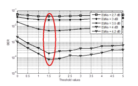Figure 3. BER (Bit error rate) performance in function of the threshold for different SNR (Signal to noise ratio) values.

Figures 4 and 5 show the simulation to determine experimentally the scaling factor for normalized minsum and minsum multi split-row, respectively, of the LDPC code (6,18) (1536,1152) . Optimal scale factor, for normalized minsum, is 0.6. And optimal scale factor, for minsum multi split-row, is 0.2.

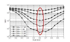Figure 4. BER (Bit error rate) performance in function of the scale factor using normalized minsum for different SNR (Signal to Noise Ratio) values.

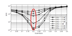Figure 5. BER (Bit error rate) performance in function of the Scale factor using minsum multi split-row for different SNR (Signal to noise ratio) values.

Figure 6 shows the simulation to determine experimentally the scaling factor for minsum threshold multi split-row of the LDPC code (6,18)(1536,1152). Optimal scale factor is 0.25 with the threshold T=1.5.

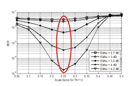Figure 6. BER (Bit error rate) performance in function of the scale factor using minsum threshold multi split-row for different SNR (Signal to noise ratio) values.

Figure 7 shows the error performance results for a (6,18) (1536,1152) LDPC code for different decoding algorithms (minsum normalized, minsum multi splitrow and minsum threshold multi split-row). The code rate is R=0.75 and the maximum number of iteration is set to I_max = 7, with threshold values obtained in Fig.3 and scale factors obtained in Fig.4, Fig.5 and

Fig.6.

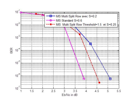Figure 7. BER performance of (6,18) (1536,1152) irregular code using various decoding algorithms.

As shown in the figure, minsum threshold multi splitrow with optimal threshold T = 1.5 performs about 0.6 dB better than minsum multi split-row and is only 0.7 dB away from MinSum normalized at BER =

6.10⁻⁷.

The minsum threshold multi split-row algorithm utilizes a threshold-enable signal to compensate for the loss of min() interpretation information in multisplit-row algorithm. It provides at least 0.6 dB error performance over the multi-split-row algorithm with Spn = 4. Partitioning the parity matrix in Spn blocs allows us to increase the decoder’s parallelism. Therefore, the partitions are performed simultaneously and we obtained a parallel decoder. That means,the complexity decreases and the decoding becomes faster.

As shown in Figure 7, the better performance gap indicated between the minsum threshold multi splitrow and minsum multi split-row algorithm revert to the information passed from one partition to another (Threshold ensp) in algorithm threshold multi splitrow, which reduces difference between the local minimum in each partition and the first and second global minimums.

4 Conclusion

In this paper we have extended threshold multi splitrow decoding method used for regular LDPC code to the irregular LDPC code. The aims was to improve the errors performances of the decoder. Simulation results show that the threshold multi split-row outperforms the multi split-row algorithm for 0.6 dB while maintaining the same level of complexity (only the comparison between the threshold and the first and second minimums is added). Our simulation results show that for a given LDPC code keeping threshold T constant at any SNR does not cause any error performance degradation.

1. G. Gallager, “Low-Density-Parity-Check,”,IRE Trans. Information Theory, vol. II, no. 8, pp. 21-28, Jan 1962.
2. MacKay et R. M. Neal, “Near Shanon Limit Performance of Low-Density-Parity-Check Codes,” ,Electron. Lett., vol. 32, pp. 1645-1946, Aug. 1996
3. J. C. MacKay, “Good error-correcting codes based on very sparse matrices,”,IEEE Trans. Inform. Theory, vol. 45, p. 399-432, Mar. 1999.
4. “IEEE 802.3an, standard for information technologytelecommunications and information exchange between systems”.
5. Cohen, A.E., Parhi and K.K,“A Low-Complexity Hybrid LDPC Code Encoder for IEEE 802.3an (10GBase- T) Ethernet,”,IEEE Transactions on Signal Processing, vol. 57, no. 10, pp. 4085-4094, 2009.
6. “T.T.S.I. digital video broadcasting (DVB) second generation framing structure for broadband satellite applications,”[ Online].
7. -M. Kim, C.-S. Park and S.-Y. Hwang,“A Novel Partially Parallel Architecture for High-Throughput LDPC Decoder for DVB-S2,”,IEEE Transactions on Con-sumer Electronics, vol. 56, no. 2, pp. 820-825, May 2010.
8. -L. Wang, Y.-L. Ueng, C.-L. Peng and C.-J. Yang, “A Low-Complexity LDPC Decoder Architecture for WiMAX Applications,”,in Proc. of the Int. Symp on VLSI Design, Automation and Test, Hsinchu, April 2011.
9. -W. Shin and H.-J. Kim,“A Multi-Mode LDPC Decoder for IEEE 802.16e Mobile WiMAX,”, Journal of Semiconductor Technology and Science, vol. 12, no. 1, pp. 24-33, Mar. 2012.
10. ElAlami and M. Mrabti,“Reduced Complexity of Decoding Algorithm for Irregular LDPC Codes Using a Multiple Split Row Method,”, International Journal of Research and Reviews in Mechatronic Design and Simulation, vol. 1, no. 1, pp. 12-17, March 2011.
11. ElAlami, H. Qjidaa, Y. Mehdaoui and M. Mrabti,“A Thresholding Algorithm for Improved Split-Row Decoding Method of Irregular LDPC Codes,”,in Proc. Of the The IEEE International Conference on Intelligent Systems and Computer Vision 2015, Fez, Morocco, March 2015.
12. Fossorier, M. Mihaljevic and H. Imai,“Reduced Complexity Iterative Decoding of Low-Density Parity-Check Codes Based on Belief Propagation,”, IEEE Transactions on Communications, vol. 47, no. 5, pp. 673-680, May 1999.
13. Mohsenin T, Baas B.“Split-row: a reduced complexity, high throughput LDPCdecoder architecture,”, Proceedings of the ICCD, October. 2006.
14. Chen and M. Fossorier,“Near optimum universal belief propagation based decoding of low-density parity check codes,”, IEEE Transaction Communications, vol. 50, pp. 406-414, Mar. 2002.
15. Chen, A. Dholakia, E. Eleftheriou, and M. Fossorier,“Reduced complexity decoding of LDPCcodes,”,IEEE Transaction Communications, vol. 53, pp. 1288-1299, Aug. 2005.
16. ElAlami, M. Mrabti and C. B. Gueye,“Reduced Complexity of Decoding Algorithm for Irregular LDPC Codes Using a Split Row Method,”,Journal of Wireless Networking and Communications, vol. 4, no. 2, pp. 29-34, 2012.
17. Mohsenin, D. Truong, and B. Baas, “Multi-splitrow threshold decoding implementations for LDPC codes,” in Proc. ISCAS, May 2009,pp. 2449-2452.

(Click to view)

(Click to view)