Introduction

The study of the flow of fluids in porous media of variable saturations is of practical interest in many fields, in agriculture, civil engineering as well as environment. Control of the movement of fluids in industrial waste, tailings and municipal waste sites requires a thorough knowledge of the dynamics of these fluids; either to assess the extent of the damage, or to design retention or containment structures or to implement a rehabilitation strategy.
It is not always technically easy to represent the physical reality of these problems in the laboratory or to design models at a reasonable cost. The mathematical and numerical modeling of the flow of fluids in porous media has for some decades made considerable progress in the wake of the rapid development of the means of calculation. The flow is modeled by nonlinear partial differential equations. These equations rarely have analytical solutions, or at the cost of simplifications which make the model without practical interest. It is rather by the various numerical approximation methods that these equations are solved. The nonlinear character of the properties of the porous media of variable saturation, the high heterogeneity of these media and the mixed nature of certain boundary conditions such as those prevailing on the soil-atmosphere interface, make the problem singularly difficult and require the implementation of robust and efficient approximation methods.
In this study, we propose a mixed formulation in volumetric water content and in interstitial pressure head. The time discretization is performed with an implicit Euler scheme with variable time step. In space, a finite element method is used. The nonlinear problem is solved by the method of successive iterations. Although the method is of the first order, taking into account the variations of the volumetric water content in the iterative scheme makes it possible to obtain the convergence with a good conservation of the mass.

As applications, we first propose the study of the classic problem of infiltrations of water in a very dry environment. It is a question of testing the convergence and the robustness of the proposed method in comparison with the results of the literature. Subsequently, the case of flow in a heterogeneous medium is examined. We study more precisely the flow of water in a medium formed of several layers of materials of different textures. The flow conditions through these layers are often complex due mainly to the non-linear behavior of the various hydraulic variables of the medium and their discontinuity in the passage from one layer to the other. Due to the contrast of the saturation state between the layers, a capillary barrier effect occurs at their interface. This can greatly reduce the movement of fluids (water and air) between layers. This mechanical phenomenon has been extensively exploited in the design of recovery systems for storage sites of various types of waste (industrial, mining, domestic, etc.). These systems contribute to the isolation of these releases from their immediate environment by restricting the movement of water and oxygen. The general characteristics of multi-layer barriers have been dealt with extensively in the mining and geotechnical literature see [1-4].

Equations of flow

Unsaturated subsurface media are triphase: the medium skeleton is the solid phase, water and air form the liquid and gaseous phases, respectively. When the skeleton is assumed to be rigid and immobile, and air is at atmospheric pressure, the flow of water is governed by Richards’ equation [5] . It is a simple (seemingly) equation model describing the evolution of volumetric water content in unsaturated soils. The Richards equation is obtained from the law of conservation of the mass of water and a law of behavior, the law of Darcy [6]. The Richards equation in a mixed formulation, volumetric water content and interstitial pressure head, is:
{■(∂θ/∂t+∇∙u=f& @ &in Ω (2.1)@u=-K(∇h+∇z)& )┤
Where Ω is a domain of the plane R^2 (or the space R^3) representing (geometrically) the porous medium, θ is the volumetric water content ([L^3 L^(-3) ] dimensionless), u is the Darcy velocity [L T^(-1) ], h is the interstitial pressure head [L], f is a source function [T^(-1) ] and z is the elevation [L]. K is the hydraulic conductivity tensor [L T^(-1) ] of the medium that is written in the form:
K=K^A K=K^A k_s k_r
Where K^A is the anisotropy tensor, K is the hydraulic conductivity, k_s is the hydraulic conductivity of the medium at water saturation and k_r is the relative conductivity.
To the equation (2.1) are associated constitutive relationships between the volumetric water content and the interstitial pressure head on the one hand, and between the hydraulic conductivity and the interstitial pressure head on the other hand. These are empirical relationships such as those proposed by [7], Van Genuchten at 1980:
θ(h)={■(θ_r+(θ_s-θ_r)/[1+|αh|^n ]^m &h<0& @ & & (2.2)@θ_s&h≥0& )┤
and
K(h)={■(k_s k_r& h<0& @ & & (2.3)@k_s& h≥0& )┤
with:
k_r=〖S_c〗^(1⁄2) [1-(1-〖S_c〗^(1⁄m) )^m ]^2, m=1-1/n for n>1, and S_c=(θ-θ_r)/(θ_s-θ_r )
Where: θ_r is the residual water content and θ_s is the water content at saturation.
Note 1:
In the literature, the Richards equation is also written and studied in a so-called interstitial pressure formulation. To obtain this formulation, we put: C(h)=∂θ/∂h, thus equation (2.1) becomes:
{■(C(h) ∂θ/∂t+∇∙u=f& @ & in Ω@u=-K(∇h+∇z)& )┤
where: C(h) is the hydraulic capacity function of the medium. In order to solve mathematically the partial differential equation (2.1), it is associated with initial and boundary conditions.

Initial conditions

We suppose that:
h(x,z,0)=h_0 (x,z) in Ω
where: h_0 is a given function on Ω.
Boundary conditions
We can associate to the equation (2.1) several types of boundary conditions according to the physical model studied:
Dirichlet boundary conditions
h(x,z,t)=h_D (x,z,t) on Γ_D×R_+
Neumann boundary conditions
-[K(∇h+∇z)]∙n=σ_n (x,z,t) on Γ_N×R_+
Gradient boundary conditions
-[K ∇h)]∙n=σ_G (x,z,t) on Γ_G×R_+
where: Γ_D, Γ_N and Γ_G are respectively parts of the boundary of the domain Ω and h_D, σ_n and σ_G are given functions and n is the normal external to Γ_N and Γ_G. In flow models across soils of varying saturation, boundary conditions are not reduced to the previous types. Non-standard conditions are imposed as seepage boundary conditions, atmospheric boundary conditions, and free drainage boundary conditions.
The seepage boundary conditions consist in imposing the interstitial pressure head at atmospheric pressure on parts Γ_S, a priori unknown, of a surface, subject to a potential seepage.
h=0 on Γ_S×R_+
The atmospheric boundary conditions are applied to the surface of the soil to take into account the physical phenomena of precipitation and evaporation on the surface Γ_A. These conditions must respect the constraints of the state of saturation or not of the soil in the vicinity of the surface in the form of the two inequalities:
|K(∇h+∇z)∙n|≤E_S on Γ_A×R_+
and
h_A≤h≤0 on Γ_A×R_+
where: E_S is the maximum potential flux on the surface and h_A is the minimum pressure head under current soil conditions.
The boundary conditions of free drainage consist in imposing the Neumann condition with: σ_G (x,z,t)=0.

Discretization

There is a vast literature on the numerical study of the Richards equation, both with the finite difference method and with finite element method see [8-15].
The finite element method has the advantage of taking into account general boundary conditions and allows to study the equation of the flow in complex geometries. In addition, the finite element method is flexible and practical.
The main difficulty of the numerical resolution of the Richards equation is its nonlinearity in h by the volumetric water content θ(h) and the hydraulic conductivity K(h) on the one hand, and the discontinuities due to heterogeneity of the environment on the other hand. Numerical methods present convergence difficulties as soon as these functions undergo sudden transitions in the vicinity of certain values of the interstitial pressure head. This is the case, for example, during the propagation of the wetting front in dry soil. The solutions exhibit instabilities with bad mass conservation see [9, 16, 17].
In the literature, the Richards equation is written and discretized under three types of formulations: in h, in θ and in h and θ. These formulations are formally identical, but sometimes produce different numerical results [18-20]. The formulation in h does not ensure a good conservation of the mass unless we consider a fine mesh and a small time step. The formulation in θ gives a very good conservation of the mass [9], but it does not make it possible to treat correctly the flow in the saturated zones, because the equation degenerates. The so-called mixed form in h and θ, for its part, ensures a good approximation of the solution and a better conservation of the mass. A discussion of this subject in the one-dimensional case is found in [9], [18]. The choice of iterative methods, such as Newton-Raphson or the method of successive approximations (Picard) as well as their various variants, also depends on the considerations of the cost in computation time.
In this section, we study the approximation of the solutions of the Richards equation. We use a finite difference scheme for time discretization with a variable time step. On each time step, we obtain a nonlinear stationary problem, which is solved after linearization by an iterative method. At each iteration, a linear problem is solved by a standard finite element method.

Time discretization

In the following, we present the time discretization of the Richards equation in the so-called mixed form h and θ:
∂θ/∂t-∇∙[K(h)(∇h+∇z)]=f (3.1)
We denote by ∆t the time step and by t_0,t_1,…,t_n,t_(n+1),… the points of the discretization, with t_(n+1)=t_n+∆t. We also denote by h^n, θ^n and f^n respectively the values of h, θ and f at time t_n, ie h^n=h(∙,t_n), θ^n=θ(h(∙,t_n)) and f^n=f(∙,t_n). The discretization of (3.1) by the implicit Euler scheme leads us to solve the nonlinear problem, finding h^(n+1) satisfying:
{■((θ^(n+1)-θ^n)/∆t-∇∙[K(h^(n+1) ) (∇h^(n+1)+∇z)]=f^(n+1)& in Ω& @h^(n+1) (x,z)=h_D (x,z,t_(n+1) ) & on Γ_D& (3.2)@-K(h^(n+1) ) (∇h^(n+1)+∇z)∙n=σ_N (x,z,t_(n+1) ) & on Γ_N& )┤
To be able to write an iterative scheme of successive approximations of this problem, we must first linearize the function θ(h). If we denote by h^(n+1,ϑ), h^(n+1,ϑ+1) the ϑ+1 th and ϑ th approximation of h^(n+1), we then write using the Taylor formula :
θ^(n+1,ϑ+1)-θ^(n+1,ϑ)=θ(h^(n+1,ϑ+1) )- θ(h^(n+1,ϑ) )≈dθ/dh (h^(n+1,ϑ) ) (h^(n+1,ϑ+1)- h^(n+1,ϑ) ) (3.3)
or
θ^(n+1,ϑ+1)-θ^(n+1,ϑ)=θ(h^(n+1,ϑ+1) )- θ(h^(n+1,ϑ) )≈C(h^(n+1,ϑ) ) (h^(n+1,ϑ+1)- h^(n+1,ϑ) ) (3.4)
The linearization of (3.2) is written in the form
{■(C(h^(n+1,ϑ) ) (h^(n+1,ϑ+1)- h^(n+1,ϑ))/∆t-∇∙[K(h^(n+1,ϑ) ) (∇h^(n+1,ϑ+1)+∇z)]=f^(n+1)-(θ^(n+1,ϑ)- θ^n)/∆t&in Ω& @h^(n+1,ϑ+1) (x,z)=h_D (x,z,t_(n+1) ) &on Γ_D&(3.5)@-K(h^(n+1,ϑ) ) (∇h^(n+1,ϑ+1)+∇z)∙n=σ_N (x,z,t_(n+1) ) &on Γ_N& )┤
The iterative process (3.5) is called by some authors a method of modified Picard iterations [9, 18].
Note 2:
In the equation (3.2) we could have linearized the function K(h^(n+1)), as we did for θ(h^(n+1)), by writing its Taylor expansion to the order 1 in the neighborhood of a given approximation h^(n+1,ϑ), which will naturally involve the derived from dK/dh. This would lead to an iterative second order scheme of the Newton type. From this point of view, scheme (3.5) appears in fact as an approximation of Newton’s method. The use of the Newton method is advantageous in the case of very dry soils where it converges faster, but with a higher cost [18].
Finite element discretization
We decompose the domain of the flow Ω into a finite number of elements. The approximate resolution of (3.5) by the finite element method in a standard Galerkin type formulation consists in determining the solution h^(n+1,ϑ+1) in the form:
h^(n+1,ϑ+1)=∑_(j=1)^nn▒〖φ_j h_j^(n+1,ϑ+1) 〗
Where: nn denotes the number of interpolation nodes, {φ_1,…,φ_nn } are the basic functions of the Lagrange interpolation space, and h_j^(n+1,ϑ+1) is the degree of freedom of h_i^(n+1,ϑ+1) at the jth node. Galerkin’s method amounts to writing that h_i^(n+1,ϑ+1) verifies (3.5) in the weak sense, that is, the integral identity:
∫_Ω^ ▒{C(h^(n+1,ϑ) ) (h^(n+1,ϑ+1)- h^(n+1,ϑ))/∆t φ_i+K(h^(n+1,ϑ) ) ∇h^(n+1,ϑ+1)∙∇φ_i+K(h^(n+1,ϑ) ) ∇z∙∇φ_i+(θ^(n+1,ϑ)- θ^n)/∆t φ_i-f^(n+1) φ_i }dΩ=∫_(Γ_N)^ ▒〖σ_N φ_i dΓ〗 (3.6)
for any basic function φ_i.
By introducing the explicit form of the terms of identity (3.6), we obtain the linear systems.
[([M^(n+1)])/Δt+[A^(n+1) ]] {h^(n+1,ϑ+1) }={Q^(n+1) }
where: [M^(n+1)] is the mass matrix given by:
M_ij^(n+1)=∫_Ω^ ▒〖C(h^(n+1,ϑ) ) φ_i φ_j dΩ〗
[A^(n+1)] is the stiffness matrix
A_ij^(n+1)=∫_Ω^ ▒〖K(h^(n+1,ϑ) ) 〖∇φ〗_i∙ ∇φ_j dΩ〗
end the vector Q^(n+1) is given by
Q_ij^(n+1)=∫_Ω^ ▒〖{f^(n+1) φ_i-K(h^(n+1,ϑ) ) ∇z∙∇φ_i } dΩ〗+ 1/∆t ∫_Ω^ ▒〖{C(h^(n+1,ϑ) )(h^(n+1,ϑ) )-θ^(n+1,ϑ)+ θ^n } φ_i dΩ〗+∫_(Γ_N)^ ▒〖σ_N φ_i dΓ〗
for : i,j = 1,nn.
We have thus reduced the approximation of the problem (2.1) to the resolution of a linear system of type (3.7) on each time step.
Resolution algorithm
Given t_max the maximum time of the simulation, and 〖∆t〗_min≤∆t≤〖∆t〗_max the interval of the time steps
Given N the maximum number of non-linear iterations
Given ε and δ respectively the tolerances on the interstitial pressure head and the volumetric water content
Loop on the time steps: t=〖t 〗_(n+1) ,t_(n+2) ,… ,t_max
Loop on non-linear iterations: ϑ=0,1,…,N
For ϑ=0, put h^(n+1,0)=h^n
Calculate h^(n+1,ϑ+1) solution of the linear system [([M^(n+1)])/Δt+[A^(n+1) ]] {h^(n+1,ϑ+1) }={Q^(n+1) }
If ‖h^(n+1,ϑ+1)-h^(n+1,ϑ) ‖≤ε and ‖θ^(n+1,ϑ+1)-θ^(n+1,ϑ) ‖≤δ
Convergence achieved on non-linear iterations
To pose : h^(n+1)=h^(n+1,ϑ+1)
Return to step 3 with 〖t=t〗_(n+2)
If the maximum number of iterations on N is reached
Convergence not achieved in N iterations
Reduce time step
Return to step 3 with 〖t=t〗_(n+1)
Note:
The test on θ (step (7)) allows a better control of the volumetric water content and ensures a better convergence and conservation of the mass.

Linear system resolution

The linear system obtained in (3.7) is of the form: Ax =b, where A is a symmetric and definite positive sparse matrix N×N, and b is a vector of R^N given, x is the unknown vector of R^N. When Matrix A is small, the system can be solved by a direct method such as the Gauss or Choleski elimination method. If, on the other hand, A is large, it is more advantageous to use iterative methods such as the conjugate gradient method or the preconditioned conjugate gradient method. In our case, we use the conjugate gradient method preconditioned by incomplete LU factorization [21].

Numerical simulations

In this section, some examples of flow tests in porous media are presented. The main aim is to demonstrate the effectiveness of the formulation used and the robustness of the finite element method. This is particularly illustrated in the case of water infiltration in very dry porous media as well as in the case of drainage in heterogeneous media.
Infiltration in a homogeneous column
The classical problem of infiltration of water into a homogeneous porous column is considered. This example has been widely used by several authors to validate their numerical methods for solving flow problems in porous media of variable saturation. See [9, 18, 20, 22, 23, 24]. The hydraulic properties of the medium are:
θ_r θ_s α k_s (cm/s)
0,102 0,368 0,0335 0,00922
Figures 1 and 2 show the characteristics of the medium, θ(h) and K(h).

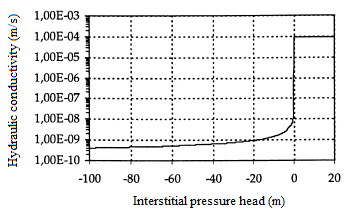Figure 1: Hydraulic conductivity

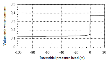Figure 2: Volumetric water content

In this first test, the height of the column is L=30 cm. The initial condition is h(.,0)=- 1 000 cm, while the boundary conditions are h(L,t)=- 75 cm at the surface of the column and h(.,0)=- 1 000 cm on its base. The simulation time is 6 hours. A regular mesh has been produced with the height of the elements ∆z=0,25 cm. It has been used with several time steps, from the finest ∆t=0,1 s to the widest 50 s≤∆t≤500 s. The solutions obtained are quite comparable to those of Lehmann in [18], and to the semi-analytical solution of Philip [25] as well as those obtained by [9]. We also considered a fine mesh with elements of size ∆z=0,1 cm and a time step ∆t=0,1 s. This mesh was used to calculate the comparison solution. In the case of the fine mesh and the small time step, the same results are obtained with a good conservation of the mass. In figures 3 and 4, the curves of the interstitial pressure head and the curves of the volumetric water content as a function of the elevation for a regular mesh, whereas in figures 5 and 6 the same representations in the case of fine mesh.

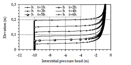Figure 3: Interstitial pressure head

(regular mesh ∆z=0,25 cm)

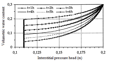Figure 4: Interstitial pressure head

(regular mesh ∆z=0,25 cm)

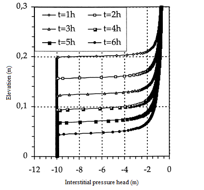Figure 5: Interstitial pressure head

(fine mesh ∆z=0,1 cm)

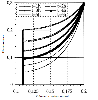Figure 6: Volumetric water content

(fine mesh ∆z=0,1 cm)
Figure 7 shows the curve of the interstitial pressure head as a function of the calculated elevation and the curve of the semi-analytical solution of Philip [25].

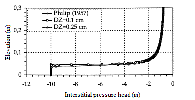Figure 7: Interstitial pressure head (regular mesh, fine mesh and Philip [25])

Infiltration in a heterogeneous (multilayer) column
An example given by Lehman in [18]. It is a heterogeneous column of height L=180 cm. In this example, it is sought to test the hydraulic behavior of a heterogeneous medium with boundary conditions relating to a wetting and drainage cycle. The porous medium consists of three layers each 60 cm thick. The hydraulic parameters of the first and the third layer (Berino loamy fine sand) and those of the second layer (Glendale clay loam) are given by:
Table 1: Hydraulic parameters of the first and the third layer
Berino loamy fine sand Glendale clay loam
θ_r 0,0286 0,1060
θ_s 0,3658 0,4686
α cm^(-1) 0,0280 0,0104
n 2,239 1,3954
k_s (cm/j) 541 13,1
The characteristics of the medium, θ(h) and K(h) are shown in figures 8 and 9.

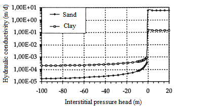Figure 8: Hydraulic conductivity

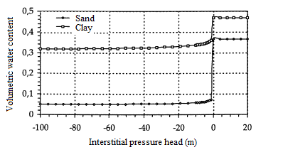Figure 9: Volumetric water content

At the top of the column, atmospheric boundary conditions are predicted with precipitation and evaporation, figure 10.

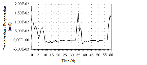Figure 10: Precipitation and Evaporation

Free drainage conditions are imposed at the bottom of the column. Two types of tests were carried out: a first test with the initially wet medium and a second initially dry test.

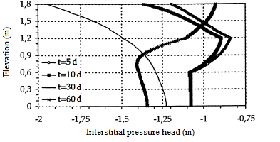Figure 11: Interstitial pressure head

(fine mesh h(∙,0)=-100 cm)

I) Initially wet medium

The initial interstitial pressure head is taken as h(.,0)=-100 cm. We first considered a regular mesh, with the height of elements ∆z=5,0 cm. For the time steps, 0,01≤∆t≤1,0 was used. Thereafter, a mesh with element height ∆z=1,0 cm was used. In both cases, we find the same results as Lehman and al. [18], figures 11 and 12. In figure 12, it is noted that the middle layer has been saturated rapidly, while the top and bottom layers desaturate. Thus we are in the presence of an effect of capillary barrier between layers.

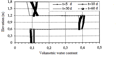Figure 12: Volumetric water content

(fine mesh h(∙,0)=-100 cm)

II) Initially dry medium

For this test, it is assumed that the three media are initially very dry. The initial interstitial pressure head is taken as h(.,0)=-10 000 cm and as a time step, successively ∆t=0,1 days and ∆t=1,0 days. To obtain good convergence, we have considered the fine mesh (∆z=1,0 cm) associated with a rather small time step (∆t=0,0001 days). Figures 13 and 14 shows the interstitial pressure head and the volumetric water content. As in the previous case, a capillary barrier effect is highlighted. Although the medium was initially dry h=-10 000 cm, the layer of fine material in the middle of the column saturates quite rapidly, while that of the top remains slightly saturated and that of the bottom always dry, figure 14.

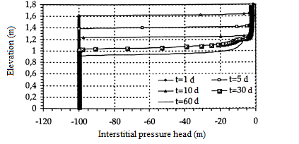Figure 13: Interstitial pressure head
(fine mesh h(∙,0)=-10 000 cm)

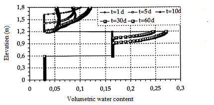Figure 14: Volumetric water content

(fine mesh h(∙,0)=-10 000 cm)

4.3. Drainage in a heterogeneous column (dry barriers)

This is an example of covers with capillary barrier effects from the authors’ work in [26]. An initially saturated multilayer medium is drained. The layers are of materials with highly contrasted hydraulic properties. The values of the parameters characterizing the covering materials are:
Sand Unreactive mining rejection
θ_r 0,0490 0,0456
θ_s 0,39 0,41
α cm^(-1) 0,0290 0,0017
n 10,2100 2,1366
k_s (cm/j) 2,10×10-2 6,58×10-5
The geometry is a vertical column of height n=110 cm containing a layer of unreactive mining rejection (fine silty material) 60 cm thick confined between two layers of sand (coarse material) 30 cm thick for the bottom layer and of 20 cm thick for the top layer. The medium was initially saturated (the interstitial pressure head was zero everywhere), thereafter a free drainage condition was imposed at the base of the column. The simulation is 60 days. Both layers of sand drain very quickly, figure 15. On the second day, the water content and pressure curves stabilized. The volumetric water content of the fine layer remains substantially at its saturation value, figure 16.

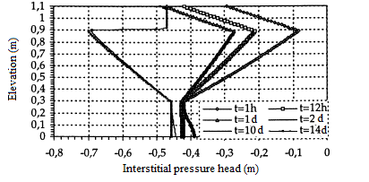Figure 15. Interstitial pressure head

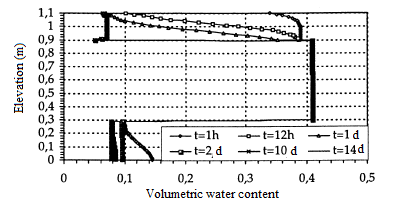Figure 16. Volumetric water content

5. Conclusion

A finite element method has been developed for calculating the distribution of the interstitial pressure head and the volumetric water content in a water flow through a heterogeneous porous medium such as soil with variable saturation and initially dry. In the resolution, boundary conditions close to the actual conditions are taken into account. In particular, mixed-type conditions corresponding to atmospheric conditions on the soil surface. Conventional flow tests in the columns have proved the robustness and stability of the method with good conservation of the mass.
References

1. Bussière, M. Idrissi, N.E. Elkadri, M. Aubertin, “Simulation des écoulements dans les milieux poreux de saturation variable à l’aide de la formation mixte de l’équation de Richard” Proceedings 1st joint IAH-CNC-CGS groundwater speciality conference, 335-342, 2000.
2. J. Morel-Seytoux, “Capillary Barrier at the Interface of Two Layers” Water Flow and Solute Transport in Soils, 20, 136-151, 1993.
3. Pabst, M. Aubertin, B. Bussière, J. Molson, “Experimental and numerical evaluation of single-layer covers placed on acid-generating tailings” Geotechnical and Geological Engineering. 35(4), 1421-1438, 2017.
4. Ross, “The diversion capacity of capillary barriers”, Water Resources research, 26(10),  2625-2629,1990.
5. A. Richards, “Capillary conduction of liquids through porous medium. Physics”, 1, 318-333, 1931.
6. Bear, “Dynamics of porous media”, Dover Publications, New York. 1988.
7. Mualem, “A new model for predicting the hydraulic conductivity of unsaturated porous media”, Water Resources research, 12(3), 573-522, 1976.
8. Belfort, F. Lehmann, “Comparison of equivalent conductivities for numerical simulation of onedimensional unsaturated flow”, Vadose Zone Journal, 4, 1191-1200, 2005.
9. A. Celia, E.T. Bouloutas, R.L. Zarba, “A general mass-conservative numerical solution for the unsaturated flow equation”,  Water resources research,  26(7), 1483-1496, 1990.
10. Haverkamp, M. Vauclin, J. Touma, P.J. Wierenga, G. Vachaud, “A comparison of numerical simulation models for one-dimensional infiltration”, Soil Science Society of America Journal, 47, 285-294, 1977.
11. W. Farthing, C. E. Kees, C. T. Miller, “Mixed finite element methods and higher order temporal approximations for variably saturated groundwater flow”, Advances in Water Resources, 26(4), 373-394, 2003.
12. Mousavi Nezhad, A. A. Javadi, F. Abbasi,“Stochastic finite element modelling of water flow in variably saturated heterogeneous soils”, International journal for numerical and analytical methods in geomechanics, 35, 1389-1408, 2011.
13. Rees, I. Masters, A.G. Malan, R.W. Lewis, “An edge-based finite volume scheme for saturated unsaturated groundwater flow”, Computer Methods in Applied Mechanics and Engineering, 193, 4741-4759, 2004.
14. E. Serrano “Modeling infiltration with approximate solutions to Richard’s equation”, Journal of Hydrologic Engineering, 9(5), 421-432, 2004.
15. Vanderborght, R. Kasteel, M. Herbst, M. Javaux, D. Thiery, M. Vanclooster, C. Mouvet , H. Vereecken, “A set of analytical benchmarks to test numerical models of flow and transport in soils”, Vadose Zone Journal,  4(1),  206-221, 2005.
16. Hao, R. Zhang, A. Kravchenko, “A mass-conservative switching method for simulating saturated-unsaturated flow”, Journal of Hydrology, 311( 1-4),  254-265, 2005.
17. Kosugi, “Comparison of three methods for discretizing the storage term of the Richards equation”, Vadose Zone Journal, 7(3),  957-965, 2008.
18. Lehmann, PH. Ackerer, “Comparison of iterative methods for improved solutions of fluid flow equation in partially saturated porous media”, Transport in Porous Media, 31,  275-292, 1998.
19. Paniconi, M. Putti, “A comparison of Picard and Newton iteration in the numerical solution of multidimensional variably saturated flow”, Water Resources research, 30 (12),  3357-3374, 1994.
20. Rathfelder, L. M. Abriola “Mass conservative numerical solutions of the head based Richards equation”, Water Resources research, 39(9),   2579-2586, 1994.
21. G. Ciarlet, “Introduction à l’analyse numérique matricielle et à l’optimisation. Masson”, 1985.
22. Haverkamp, M. Vauclin, J. Touma, P. J. Wierenga, G. Vachaud, “A comparison of numerical simulation models for one-dimensional infiltration”, Soil Science Society of America Journal, 47,  285-294, 1977.
23. Touma, M. Vauclin, “Experimental and numerical analysis of two-phase infiltration in a partially saturated soil”, Transport in Porous Media, 1,  22-55, 1986.
24. Vauclin, “Flow of water and air in soils: Theoretical and experimental aspects, in unsaturated flow in hydrologic modeling, Theory and Practice”, edited by H. Morel-Seytoux,  53-91, Kluwer Academic, Dordrecht,  Netherlands, 1989.
25. R. Philip, “The theory of infiltration: 1. The infiltration equation and its solution”, Soil Sci., 83, 435-448, 1957.
26. Aachib, M. Aubertin, R. P. Chapuis, “Essais en colonne sur des couvertures avec effets de barrière capillaire”, 51ème conférence canadienne de géotechnique,  2, Edmonton, 1998.

(Click to view)

(Click to view)