1. Introduction

In the automative industry, many workpieces such gears, bearings, racks and pinions, are made of steel. Steel is an alloy of iron and carbon. Generally, indus-trial steel has a carbon content up to about 2 wt%. Other alloying elements may be present, such as Cr and V in tools steels, or Si, Mn, Ni and Cr in stain-less steels. Most structural components in mechanical engineering are made of steel. Certain of these com-ponents, such as toothed wheels, bevel gears, pinions and so on, engaged each others in order to transmit some kind of (rotational or longitudinal) movement. In this situation, the contact surfaces of these compo-nents are particularly stressed. The goal of heat treat-ing of steel is to attain a satisfactory hardness. Prior to heat treating, steel is a soft and ductile material. Without a hardening treatment, and due to the sur-face stresses, the gear teeth will soon get damaged and they will no longer engage correctly.

In this work we are interested in the mathematical description of the hardening procedure of a car steer-ing rack (see Figure 1). This particular situation is one of the major concerns in the automotive industry. In this case, the goal is to increase the hardness of the steel along the tooth line and at the same time keep-ing the rest of the workpiece soft and ductile in order to reduce fatigue. This problem is governed by a non-linear system of partial differential equations coupled with a certain system of ordinary differential equa-tions. Once the full system is set we perform some numerical simulations.

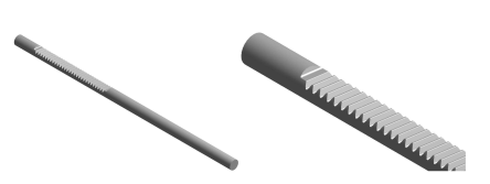Figure 1: Car steering rack.

Solid steel may be present at different phases, namely austenite, martensite, bainite, pearlite and fer-rite. The phase diagram of steel is shown in Fig-ure 2. For a given wt% of carbon content up to 2.11, all steel phases are transformed into austenite pro-vided the temperature has been raised up to a cer-tain range. The minimum austenization temperature (727 ) is attained for a carbon content of 0.77 wt% (eutectoid steel). Upon cooling, the austenite is trans-formed back into the other phases (see Figure 3), but its distribution depends strongly on the cooling strategy ([4, 12]).

Martensite is the hardest constituent in steel, but at the same time is the most brittle, whereas pearlite is the softest and more ductile phase. Martensite de-rives from austenite and can be obtained only if the cooling rate is high enough. Otherwise, the rest of the steel phases will appear.

The hardness of the martensite phase is due to a strong supersaturation of carbon atoms in the iron lattice and to a high density of crystal defects. From the industrial standpoint, heat treating of steel has a collateral problem: hardening is usually accompanied by distortions of the workpiece. The main reasons of these distortions are due to (1) thermal strains, since steel phases undergo different volumetric changes during the heating and cooling processes, and (2) experiments with steel workpieces under applied loading show an irreversible deformation even when the equivalent stress corresponding to the load is in the elastic range. This effect is called transformation induced plasticity.

The heating stage is accomplished by an induction-conduction procedure. This technique has been successfully used in industry since the last century. During a time interval, a high frequency cur-rent passes through a coil generating an alternating magnetic field which induces eddy currents in the workpiece, which is placed close to the coil. The eddy currents dissipate energy in the workpiece producing the necessary heating.

2. Mathematical modeling

We consider the setting corresponding to Figure 4. The domain    ^c represents the inductor (made of copper) whereas     ^s stands for the steel workpiece to be hardened. Here, the coil is the domain = ^s [ ^c [ S₀. In this way, the workpiece itself takes part of the coil.

In order to describe the heating-cooling process, we will distinguish two subintervals forming a parti-tion of [0; T ], namely [0; T ] = [0; T_h) [[T_h; T_c], T_c > T_h >

The first one [0; T_h) corresponds to the heating pro-cess. All along this time interval, a high frequency electric current is supplied through the conductor which in its turn induces a magnetic field. The com-bined effect of both conduction and induction gives rise to a production term in the energy balance equa-tion (14), namely b( )jA_t +r j². This is Joule’s heating which is the principal term in heat production. In our model, we will only consider three steel phase frac-tions, namely austenite (a), martensite (m), and the rest of phases (r). In this way, we have a + m + r = 1

At the instant t = T_h, the current is switched off and during the time interval [T_h; T_c] the workpiece is severely cooled down by means of aqua-quenching. The heating modelbe obtained. In particular m = 0 in ^s [0; T_h] and the transformation to austenite is derived at the expense of the other phase fractions (r).

The current passing through the set of conductors

The heating model involves the following un-knowns: the electric potential, ; the magnetic vec-tor potential, A = (A₁;A₂;A₃); the stress tensor, = ( _ij )_{1 i;j 3}, _ij = _ji for all 1 i; j 3; the dis-placement field u = (u₁; u₂; u₃); the austenite phase fraction, a; and the temperature, . Among them, only A is defined in the domain D containing the set of conductors . On the other hand, since the inductor and the workpiece are in close contact, both and are defined in . Since phase transitions only occur in the workpiece, we may neglect deformations in ^c. This implies that , u and a are only defined in the workpiece ^s.

Since electromagnetic fields generated by high fre-quency currents are sinusoidal in time, both the elec-tric potential, , and the magnetic potential field, A take the form ([1, 2, 14, 15]) M(x; t) = Re e^i!tM(x) , where M is a complex-valued function or vector field, and ! = 2  f is the angular frequency, f being the electric current frequency. In general, M also depends on t, but at a time scale much greater than 1=!. In this way, we may introduce the complex-valued fields

As a far as the numerical simulation of a system like (2)-(15) is concerned, the introduction of the new variables ’ and A is quite convenient since the time scale describing the evolution of both ’ and A is much smaller than that of the temperature . In the case of steel heat treating, f is about 80 KHz. The heating model reads as follows ([3, 9, 10, 7]):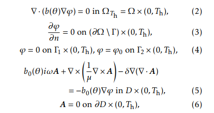

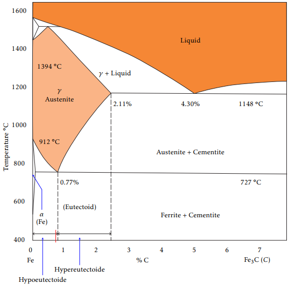Figure 2: Iron-carbide phase diagram.

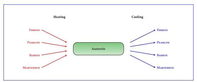Figure 3: Microconstituents of steel. Upon heating, all phases are transformed into austenite, which is transformed back to the other phases during the cooling process. The distribution of the new phases depends strongly on the cooling strategy. A high cooling rate transforms austenite into martensite. A slow cooling rate transforms austenite into pearlite.

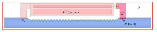Figure 4: Domains D,   =  ^s [  ^c [S₀ and the faces ₁; ₂     ^c. The inductor

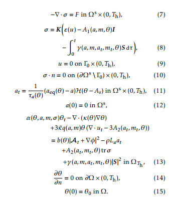Here, b( ) is the electrical conductivity (by b( ) we mean the function (x; t) 7! b(x; (x; t)), and also for ( ), etc.); ’₀ represents the potential external source. The domain D containing the set of conductors is taken big enough so that the magnetic vector potential A vanishes on its boundary @D (in our model, is taken to be a 2D rectangle or a 3D cube). Since both part to be hardened by means of the heating-cooling process described below. It is made of a hypoeutectoid steel. The domain is taken as a big enough rectangle containing both the inductor and the rack  and in its turn q_a, q_m and q_r are the thermal expan-sion coefficients of the phase fractions a, m and r, respectively, and _a, _m and _r are reference tempera-tures (notice that during the heating stage is m = 0);  ^{R t} (a; m; a_t; m_t;  )S d   gives the model, through the function , of the transformation induced plasticity strain tensor, where S = ¹₃ tr I is the deviator of , that is, the trace free part of the stress tensor; ₀ is a certain smooth enough part of @ ^s; n is the unit outer normal vector to the referred boundary; the functions _a( ), a_eq( ) are given from experimental data (see Figure 5), and H is the Heaviside function; ( ) is the thermal conductivity; the functions appearing in (13) are given as follows

and a are only defined in          ^s, when they appear in

a term referred in     , we mean that this term vanishes

outside     ^s (for instance,        L_aa_t appearing in (13));

b₀(x; s) = b(x; s) if x 2     , b₀(x; s) = 0 elsewhere;        =   (x)

is the magnetic permeability; > 0 is a small constant; F is a given external force (usually F = 0); K = K_ijkl , 1 i; j; k; l 3 is the stiffness tensor. Steel can be con-sidered as an isotropic and homogenous material so that

K_ijkl =        _{ij  kl} + ( _{ik  jl} + _{il  jk}); for all i; j; k; l 2 f1;2;3g

( ; a; m;  ) =      c_“    9 ¯q(a; m)²    q(a; m) tr  ;

where and c_“ are the steel density and the spe-cific heat capacity at constant strain, respectively, ¯ =

	1	¯
	3	(3  + 2 ¯) is the bulk modulus, and q(a; m) is defined

as

q(a; m) = q_aa + q_mm + (1    a   m)q_r ;

A₂(a_t; m_t;  ) = q_aa_t(         _a) + q_mm_t(        _m)

q_r (a_t + m_t)(        _r ):

where	¯	0 and1		¯	0	are the Lame´ coe			ffi	cients
				>			T
of steel;		“(u) =	2	(ru +		ru		) is the strain	tensor;

A₁(a; m;  )I models the thermal strain, I being the 3  3

Finally, L_a > 0 is the latent heat related to the austen-ite phase fraction. Notice that, in a more general situ-ation , c_“ and L_a may also depend on a, m and/or .

Figure 5: Functions a_eq and  _a.

Equations (2) and (5) derive from Maxwell’s equa-tions. In [9], it is assumed the Coulomb gauge condi-tion for the magnetic vector potential, namely, r A =

1. Here, we do not impose this condition since this makes appear an undesired pressure gradient in the equation for A. In its turn, we include a penalty term in this equation of the form r(r A). In doing so, both the theoretical analysis and the numerical simu-lations are simplified.

Equation (7) is a quasistatic balance law of mo-mentum and (8) is Hooke’s law. The transformation to austenite from the initial phase r(0) = 1 is described in (11).

Finally, equation (13) derives from the balance law of internal energy. As it has been pointed out above, Joule’s heating is the main responsible in heat pro-duction. Since (a; m; a_t; m_t; )jSj² 0, the contribu-tion of the transformation induced plasticity to the energy balance is also a production term. On the other hand, during the heating stage we have a_t 0 so that L_aa_t 0. This means that the transformation to austenite absorbs energy, which is released during the cooling stage.

The cooling model reads as follows

(x; t) =	0	on @	\ @	c;
(	0(t)  on @		\ @	s:

In (22) c_m > 0 is a constant value. Also, in (24), L_m > 0 is the latent heat related to the martensite phase fraction. The function (x; t) in (25) is a heat transfer coefficient and is given by

where ₀(t) > 0 (usually taken to be constant). Finally, _e is the temperature of the quenchant.

The mathematical analysis of a system similar to (16)-(26) can be seen in [3]. In this reference, an existence result is shown assuming that the data are smooth enough and T_c T_h is sufficiently small.

The heating process ends, the high frequency current passing through the coil is switched-off and aqua-quenching begins. The quenching is just modeled via the Robin boundary condition given in (25).

We put a_Th = a(T_h), that is, a_Th is the austenite phase fraction distribution at the final heating instant T_h obtained from (11). In the same way, we define _Th = (T_h). Obviously, these functions will be taken as the initial phase fraction distribution and temper-ature, respectively, in the cooling model. Here we use the Koistinen-Marburger model ([11, 13]) for the description of the transformation to martensite from austenite.

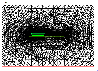Figure 6: Domain triangulation. The mesh contains 61790 trian-gles and 30946 vertices.

3. Numerical simulation

Using the Freefem++ package ([8]), we have per-formed some numerical simulations for the approxi-mation of the solution to the systems (2)-(15) and (16)-(26). We want to describe the hardening treatment of a car steering rack during the heating-cooling process. The goal is to produce martensite along the tooth line together with a thin layer in its neighborhood inside the steel workpiece ([5, 6]).

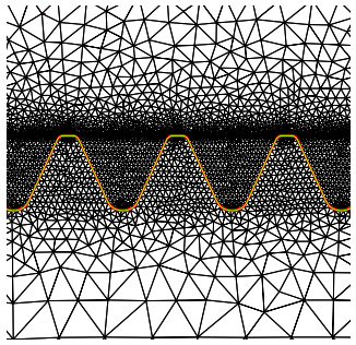Figure 7: Domain triangulation. Element density near three teeth.

Figure 4 shows the open sets D, = ^s [ ^c [ S and the faces ₁ and ₂ (they appear stick together in this figure) which intervene in the setting of the problem. The workpiece contains a toothed part to be hardened by means of the heating-cooling process described above. It is made of a hypo eutectoid steel. The open set D n ^¯ is air. The magnetic permeability in (5) is then given by

In this simulation, the final time of the heating process is T_h = 5:5 seconds and the cooling process extends also for 5.5 seconds, that is T_c = 11. We have used the finite elements method for the space approximation and a Crank-Nicolson scheme for the time discretization. Figures 6 and 7 show the triangulation of D in our numerical simulations. We have used P₂-Lagrange approximation for ’, A and and P₁ for a and m.

In Figure 8 we can see the temperature distribution of the rack along the tooth line at different in-stants of the the heating-cooling process. The initial temperature is ₀ = 300K. At t = 5:5 the heating process ends and the computed temperature shows that the temperature along the rack tooth line lies in the interval [1050;1670] (K).

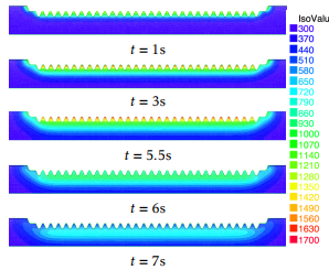Figure 8: Temperature evolution at instants t = 1, t = 3, t = 5:5 (end of the heating stage, aqua-quenching begins), t = 6 and t = 7 seconds, respectively. At t = 5:5s the temperature along the tooth part has reached the austenization level in this part of the rack. The temperature is measured in Kelvin.

The martensite phase can only derive from the austenite phase. Thus we need to transform first the critical part to be hardened (the tooth line) into austenite. For our hypo eutectoid steel, austenite only exists in a temperature range close to the interval [1050;1670] (in K). During the first stage, the workpiece is heated up by conduction and induction (Joule’s heating) which renders the tooth line up to the desired temperature. In order to transform the austenite into martensite, we must cool it down at a very high rate. This second stage is accomplished by aqua quenching.

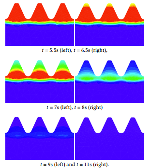Figure 9: Transformation of the austenite phase fraction during the aqua quenching at time instants t=5.5, 6.5, 7, 8, 9, and 11 seconds, respectively.

Figure 9 shows the austenite evolution from the beginning of the cooling stage.  Blue corresponds to 10% while red is 100%.  We observe that martensite starts to appear, approximatively, one second after the beginning of the cooling stage.  At the final instant, all the amount of austenite has been transformed into martensite as it is shown in Figure 10 .

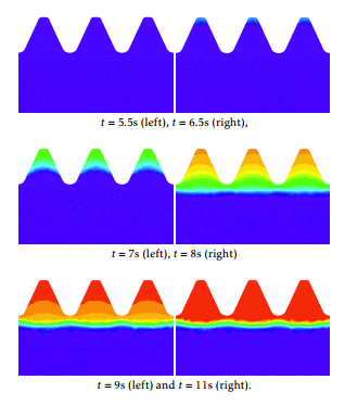Figure 10: Transformation of the martensite phase fraction from austenite during the aquaquenching at time instants t=5.5, 6.5, 7, 8, 9, and 11

Figure 11 shows the austenization along the tooth line at the end of the heating process T = 5:5 seconds.

Figure 12 shows the final distribution of martensite from austenite along the rack tooth line through the cooling stage t = 11 seconds. We have good agreement versus the experimental results obtained in the industrial process.

During the heating-cooling process,  the work piece is deformed so that an industrial rectification is needed (or otherwise the rack would be useless). Figures 13 and 14 shows the different deformations undergone by the workpiece.

Figure 11: Heating process. Austenite at t = 5:5 along the rack tooth line.

Figure 12: Cooling process. Martensite transformation at the final stage of the cooling process t = 11 seconds.

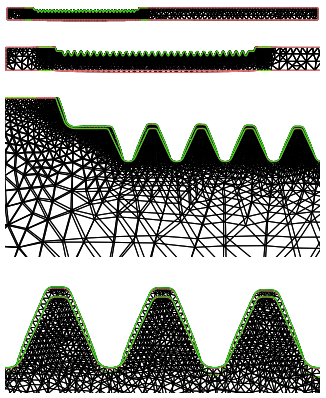Figure 13: Distorted mesh (with a scale factor of 10) after the heating stage. The austenite transformation along the tooth line changes the original profile.

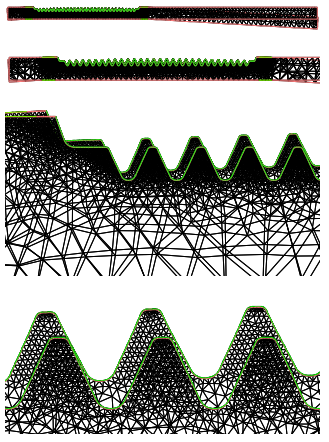Figure 14: Distorted mesh (with a scale factor of 10) after the cooling stage. The original configuration is partially recovered. Due to the plasticity effect and the lack of the upper supports, the rack bends down.

conflict of Interest The authors declare no conflict of interest.

Acknowledgments

This research was partially sup-ported by Ministerio de Educacion´ y Ciencia under grants MTM2010-16401 and TEC2014-54357-C2-2-R with the participation of FEDER, and Consejer´ıa de Educacion´ y Ciencia de la Junta de Andaluc´ıa, re-search group FQM–315.

1. Berm´ udez, J. Bull´on, F. Pena and P. Salgado, “A numerical method for transient simulation of metallurgical compound electrodes”, Finite Elem. Anal. Des., 39, 283–299, 2003. https://doi.org/10.1016/S0168-874X(02)00069-0
2. Berm´ udez, D. G´omez, M. C. Mu˜niz and P. Salgado, “Transient numerical simulation of a thermoelectrical problem in cylindrical induction heating furnaces”, Adv. Comput. Math., 26, 39–62, 2007. https://doi.org/10.1007/s10444-005-7470-9
3. K. Cheminski, D. H¨omberg and D. Kern, “On a thermomechanical model of phase transitions in steel”, Adv. Math. Sci. Appl., 18, 119–140, 2008.
4. R. Davis et al. “ASM Handbook: Heat Treating”, vol. 4, ASM International, USA, 2007.
5. M. D´iaz Moreno, C. Garc´ia V´azquez, M. T. Gonz´alez Montesinos and F. Orteg´on Gallego, “Numerical simulation of a Induction-Conduction Model Arising in Steel Hardening model arising in steel hardening”, Lecture Notes in Engineering and Computer Science, World Congress on Engineering 2009, Volume II, July 2009, 1251–1255.
6. M. D´iaz Moreno, C. Garc´ia V´azquez, M. T. Gonz´alez Montesinos, F. Orteg´on Gallego and G. Viglialoro, “Mathematical modeling of heat treatment for a steering rack including mechanical effects”, J. Numer. Math. 20, no. 3-4, 215–231, 2012. https://doi.org/10.1515/jnum-2012-0011
7. Fuhrmann, D. H¨omberg and M. Uhle, “Numerical simulation of induction hardening of steel”, COMPEL, 18, No. 3, 482–493, 1999. https://doi.org/10.1108/03321649910275161
8. Hecht, “New development in freeFem++”, J. Numer. Math. 20, no. 3-4, 251–265, 2012. https://doi.org/10.1515/jnum- 2012-0013
9. H¨omberg, “A mathematical model for induction hardening including mechanical effects”, Nonlinear Anal.-Real World Appl., 5, 55–90, 2004. https://doi.org/10.1016/S1468- 1218(03)00017-8
10. H¨omberg andW.Weiss, “PID control of laser surface hardening of steel”, IEEE Trans. Control Syst. Technol., 14, No. 5, 896–904, 2006. https://doi.org/10.1109/TCST.2006.879978
11. P. Koistinen, R. E. Marburger, “A general equation prescribing the extent of the austenite-martensite transformation in pure iron-carbon alloys and plain carbon steels”, Acta Metall., 7, 59–60, 1959. https://doi.org/10.1016/0001- 6160(59)90170-1
12. Krauss, “Steels: Heat Treatment and Processing Principles”, ASM International, USA, 2000.
13. B. Leblond and J. Devaux, “A new kinetic model for anisothermal metallurgical transformations in steels including effect of austenite grain size”, Acta Metall., 32, No. 1, 137– 146, 1984. https://doi.org/10.1016/0001-6160(84)90211-6
14. J. Pena Brage, “Contribuci´on al modelado matem´atico de algunos problemas en la metalurgia del silicio”, Ph. thesis, Universidade de Santiago de Compostela, 2003.
15. M. Yin, “Regularity of weak solution to Maxwell’s equations and applications to microwave heating”, J. Differ. Equ., 200, 137-161, 2004. https://doi.org/10.1016/j.jde.2004.01.010

(Click to view)

(Click to view)

No. of Downloads Per Month

No. of Downloads Per Country