1            Introduction

The modern 3D scanners are 3D acquisition tools which are developed in terms of resolution and acquisition speed. The clouds of points obtained from the digitization of the real objects can be very dense. This leads to an important data redundancy. This problem must be solved and optimal point cloud must be found. This optimization of the number of points results in reducing the reconstruction calculation.

The problem of simplifying point cloud can be formalized as follows: given a set of points X sampling a

0 surface S, find a sample points X with |X| ≤ |X|, Such

            0                                                                 0

that X sampling a surface S is close to S. |X| is the cardinality of set X. This objective requires defining a measure of geometric error between the original and simplified surface for which the method will resort to the estimation of the global or local properties of the original surface. There are two main categories of algorithms to sampling points: sub-sampling algorithms and resampling algorithms. The subsampling algorithms produce simplified sample points which are a subset of the original point cloud, while the resampling algorithms rely on estimating the properties of the sampled surface to compute new relevant points.

In the literature, the categories of simplification algorithms have been applied according to three main simplification schemes. The first method is simplification by selection or calculation of points representing subsets of the initial sample. This method consists of decomposing the initial set into small areas, each of which is represented by a single point in the simplified sample [1-4]. The methods of this category are distinguished by the criteria defining the areas and their construction.

The second method is iterative simplification. The principle of iterative simplification is to remove points of the initial sample incrementally per geometric or topologic criteria locally measuring the redundancy of the data [5-10].

The third method is simplification by incremental sampling. Unlike iterative simplification, the simplified sample points can be constructed by progressively enriching an initial subset of points or sampling an implicit surface [11-18].

This paper will present a hybrid simplification technique based on the entropy estimation [19] and clustering algorithm [20].

It is organized as follows: In section 2, we will recall some density function estimators. In section 3, we will present clustering algorithm. Then in section

4, we will present our 3D point cloud simplification algorithm based on Shannon entropy [21]. Section 5 will show the results and validation. Finally, we will present the conclusion.

2          Defining the Estimation of Density Function and Entropy

There are several methods for density estimation: parametric and nonparametric methods. We will fcus on nonparametric methods which include the kernel density estimator, also known as the ParzenRosenblatt method [22,23] and the K nearest neighbors (K-NN) method [24]. We will only use in this article K-NN estimator.

2.1         The K Nearest Neighbors Estimator

The algorithm of the k nearest neighbors (K-NN) [24] is a method of estimating the nonparametric probability of the density function. The degree of estimation is defined by an integer k which is the number of the nearest neighbors, generally proportional to the size of the sample N. For each x we define the estimation of the density. The distances between points of the sample and x are as follows:

r₁(x) < … < r_k−₁(x) < r_k(x) < … < r_N(x)

r_i with (i = 1…k…N) are distances sorted by ascending order.

The estimator k-NN in dimension d can be defined as follows:

                                                   k                         k

                             pknn(x) =      N          =       N                                             (1)

V_k(x)         C_dr_k(x) where r_k(x) is the distance from x to the k^th nearest point and V_k(x) is the volume of a sphere of radius. r_k(x) and C_d is the volume of the unit sphere in d dimension.

The number k must be adjusted as a function of the size N of the available sample in order to respect the constraints that ensure the convergence of the estimator. For N observations, the k can be calculated as follows:                _√

                                            k = k₀        N

By respecting these rules of adjustment, it is certain that the estimator converges when the number N increases indefinitely whatever is the value of k₀.

2.2         Defining Entropy

Claude Shannon introduced the concept of the entropy which is associated with a discrete random variable X as a basic concept in information theory [21]. The distribution of probabilities p = p₁,p₂,…,p_N associated with the realizations of X. The Shannon entropy is calculated by using the following formula:

N

X

                            H(p) = −           p(x_i)log(p(x_i))                        (2)

i=1

Entropy measures the uncertainty associated with a random variable. Therefore, the realization of the rare event provides more information about the phenomenon than the realization of the frequent event.

3          Clustering Algorithms Definition

X = {x_i ∈ R^d}, i = 1,,N is a set of observations described by d attributes; the objective of clustering is the structuring of data into homogeneous classes. Clustering is unsupervised classification. The objective is to try to group clustered points or classes so that the data in a cluster is as similar as possible. Two types of approaches are possible; hierarchical and non-hierarchical approaches[25].

In this article, we will concentrate on the nonhierarchical approach which is encapsulated in both the Fuzzy C-Means Clustering (FCM) algorithm [26,20] and K-means algorithm (KM)[27].

3.1         Fuzzy C-Means Clustering Algorithm

Fuzzy c-means is a data clustering technique wherein each data point belongs to a cluster to some degree that is specified by a membership grade. This technique was originally introduced by J.C. Dunn[20], and improved by J.C. Bezdek[26] as an improvement on earlier clustering methods. It provides a method that shows how to group data points that populate some multidimensional space into a specific number of different clusters.

X = {x₁,x₂,…,x_n} is a given data set to be analysed, and V = {v₁,v₂,…,v_c} is the set of centers of clusters in X data set in p dimensional space R^p. Where N is the number of objects, p is the number of features and c is the number of partitions or clusters. FCM is a clustering method allowing each data point to belong to multiple clusters with varying degrees of membership.

FCM is based on the minimization of the following objective function

                                              c        N

                                       Jm = XXuijmDijA2                                                   (3)

i=1 j=1

Where, D_ijA² is the distances between i^th features vector and the centroid of j^th cluster. They are computed as a squared inner-product distance norm in Equation (4):

                         D_ijA =k x_j − v_i k= (x_j − v_i)^T A(x_j − v_i)                    (4)

In the objective function in Equation (3), U is a fuzzy partition matrix that is computed from data set X:

                                               U = u_ij                                                                (5)

m is fuzzy partition matrix exponent for controlling the degree of fuzzy overlap, with m > 1. Fuzzy overlap refers to how fuzzy the boundaries between clusters are. That is the number of data points that have significant membership in more than one cluster.

The objective function is minimized with the constraints as follows: u_ij ∈ [0,1]; 1 ≤ i ≤ c; 1 ≤ j ≤

N; Pci=1uij = 1; 0 < PNi=1uij < N;

FCM performs the following steps during clustering:

1. Randomly initialize the cluster membership values, u_ij.
2. Calculate the cluster centres:

PN                 uijmxj i=1

PN              uijm i=1

.

3. Update u_ij according to the following:

1

PN (DijA/DkjA)2/(m−1)

k=1

4. Calculate the objective function, J_m
5. Compare U^(t+1) with U^(t), where t is the iteration number.
6. If k U^(t+1) − U^(t) k< ε then it stop, or else returns to the step 2. (ε is a specified minimum threshold, in this case it uses ε = 10⁻⁵).

3.2         K-Means Clustering Algorithm

The K-Means algorithm (KM) iteratively computes the cluster centroids for each distance measurement in order to minimize the sum with respect to the specified measure. The objective of the K-Means algorithm is to minimize an objective function named by squared error function given in equation (6) as follows:

                                                        c        N

                                                            XX ²                                                  (6)

                                 J_km(X;V ) =                 D_ij

i=1 j=1

D_ij² is the chosen distance measure which is in Euclidean norm: k x_ij − v_i k², 1 ≤ i ≤ c,1 ≤ j ≤ N_i. Where N_i represents the number of data points in i^th cluster. For c clusters, the K-Means algorithm is based on an iterative algorithm that minimizes the sum of the distances of each object at its cluster center. The goal is to have a minimum value of the sum of the distance by moving the objects between the clusters. The steps of K-means are as follows:

1. Centroids of c clusters are chosen from X randomly.
2. Distances between data points and cluster centroids are calculated.
3. Each data point is assigned to the cluster whosecentroid is close to it.
4. Cluster centroids are updated by using the formula in Equation (7):

XNi xij

v_i =           (7) i=1 N_i

5. Distances from the updated cluster centroidsare recalculated.
6. If no data point is assigned to a new cluster, theexecution of algorithm is stopped, otherwise the steps from 3 to 5 are repeated taking into consideration probable movements of data points between the clusters.

4          Evaulation of the Simplified Meshes

In order to give a theoretical evaluation for the simplification method, we have based on a metric of mean errors, max error and RMS(root mean square error) used by Cignoni et al.[28]. Where he measured the Hausdorff distance between the approximation and the original model. Hausdorff distance is defined as follow:

Let X and Y be two non-empty subsets of a metric space (M,d). We define their Hausdorff distance d_H = max{sup inf (d(x,y),sup inf (d(x,y))} (8) x^∈X y^∈Y y^∈Y x^∈X

In our experiments we will use the symmetric Hausdorff distance calculated with the Metro software tool[28].

In order to calculate the approximate error, we will reconstruct the models from the point clouds. We find in the literature several reconstruction techniques [29] to create a 3D model from a set of points.

In the next section, we will present our simplification approach based on the estimation of Shannon entropy and algorithm clustering. Where we will first use the FCM algorithm and then replace it with the KM algorithm and compare the results obtained from the use of the two algorithms in our simplification method. We have previously two types of nonparametric estimators, the K-NN estimator and the Parzen estimator. Each type has advantages and disadvantages. For Parzen estimator, the bandwidth choice has strong impact on the quality of estimated density [30]. For this reason, we will use K-NN estimator to estimate the density function.

5          Proposed Approach

Now, we will propose an algorithm to simplify dense 3D point cloud. First, this algorithm is based on the entropy estimation algorithm. It allows the estimation of the entropy for each 3D point of X as well as making the decision to eliminate or to keep the point. In this pproach we will use the K-NN estimator to estimate the entropy. Moreover, it is based on clustering algorithm (KM or FCM) to subdivide point cloud X into clusters in order to minimize the computation time. The procedures are:

SIMPLIFICATION ALGORITHM

• Input
  • X = {x₁,x₂,,x_N} : The data simple (point cloud)
  • S: threshold
  • c: the number of clusters
• Begin
• Decomposing the initial set of points X into c small areas denoting R_j (j = 1,2,…,c), and using clustering algorithm (FCM or KMA).
• For j = 1 to c
  • Calculate global entropy of a cluster j by using all data samples in R_j = {y₁,y₂,,y_m} according to the equation (2), Note this entropy H(R_j).
  • Calculate the entropy H(R_j − y_i) of point cloud R_j less point y_i(i = 1,2,,m)
  • Calculate 4H_i =| H(R_j) − H(R_j − y_i)| with i = 1,2,,m
  • If 4H_i ≤ S Then Rj = Rj − yi.
  • End-if
• End for End.

6          Results and Discussion

To validate the efficiency of the use of the two clustering algorithms FCM and KM in our simplification method, we use three 3D models that represent real objects such as Max Planck (fig. 1,b) and Atene (fig. 1,a). Fig. (2,a), (2,b) show simplification results on various point cloud using FCM algorithm. Fig. (3,a), (3,b) show simplification results on various point cloud using KM algorithm.

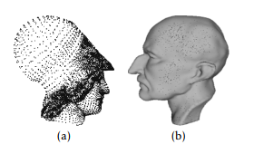Figure 1: original point cloud, a) Atene, b) Max Planck

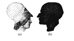Figure 2: Simplified point cloud using FCM algorithm, a) Atene, b) Max Planck

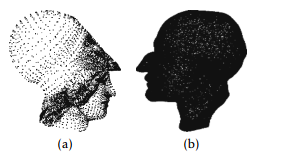Figure 3: Simplified point cloud using KM algorithm, a) Atene, b) Max Planck

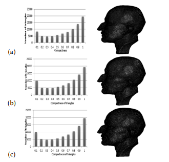Figure 4: Comparison of Max Planck mesh quality, a) Original point cloud, b) simplified point cloud using FCM, c) simplified point cloud using KM

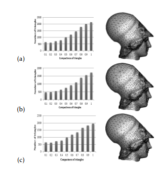Figure 5: Comparison of Atene mesh quality, a) Original point cloud, b) simplified point cloud using FCM, c) simplified point cloud using KM

In this section, we will validate the effectiveness of our proposed method. Actually, we have conducted a comparison between the original and simplified point cloud. Accordingly, we will use a comparison between the original and simplified mesh.

Thereafter, we make a comparison between the original mesh and the one created from the simplified point cloud. To reconstruct the mesh, we use ball Pivoting method [31,29] or A.M Hsaini et al. method [32]. Then, to measure the quality of the obtained meshes, we compute the quality of the triangles using the compactness formula proposed by Guziec [33]:

√

4

c =(9) l

Where l_i are the lengths of the edges of the triangle. And a is the area of the triangle. We note that this measure is equal to 1 for an equilateral triangle and 0 for a triangle whose vertices are collinear. According to [34], a triangle is an acceptable quality if c ≥ 0.6.

In figures 4, 5, we have presented the triangles compactness histogram of the two meshes. In each figure, the first line presents the reconstructed mesh from the original point cloud. The second line presents the simplified point cloud using FCM algorithm. The third line presents the simplified point cloud using KM algorithm. Note that, the evaluation of the mesh quality is achieved by the compactness of the triangles.

Depending on [34] meshes are compact if the percentage of the number of triangles, which composes mesh with compactness c ≥ 0.6 is greater than or equal to 50%. Also, according to the histograms in figures 4 and 5, it is observed that the surfaces obtained from the simplified point cloud are compact surfaces.

The table 1 also shows that the use of the KM and FCM algorithms retains the compactness of the surfaces. However, the compactness obtained by the FCM algorithm is greater than that obtained by KM for the two surfaces.

Concerning the number of vertices obtained after simplification, we note that this number is higher in the case of FCM for the two models.

It is interesting to note that in the case where FCM is used better results are produced in terms of speed. In contrast, in the other case where KM is used the speed is slow.

Table 3 and table 4 shows the numerical results obtained by the implementation of the two algorithms FCM and KM in the simplification method. The main results are average error, maximal error and root mean square error (RMS).

Figure 6 and 7 present differences between original and simplified meshes using Hausdorff distance. Note that it is a red-green-blue map, so red is minimal and blue is maximal, so in our case red means zero error and blue high error.

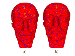Figure 6: difference between original and simplified MaxPlanck mesh

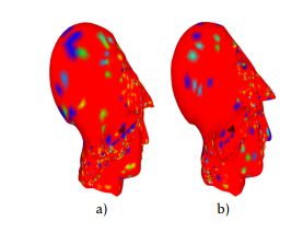Figure 7: difference between original and simplified Atene mesh

Table 3 presents the results relative to the evaluation of the approximation error concerning MaxPlanck model. Table 4 Also presents the same error related to Atene model.

Table 1: simplification results with s=0.001 using KM algorithm Object Number of points Number of cluster KM com- putation time (s) Percentage of triangles with a compactness ≥ 0.6 (%)   Original Simplified using KM Simplified using KM Original Atene 6942 6289 18 1118.98 57.85 59.84 max planck 49089 44765 123 7752.49 58.54 59.45 Table 2: simplification results with s=0.001 using FCM algorithm Object Number of points Number of cluster FCM compu- tation time (s) Percentage of triangles with a compactness ≥ 0.6 (%)   Original Simplified using FCM Simplified using FCM Original Atene 6942 6289 18 775.75 60.19 59.84 max planck 49089 44812 123 7356.52 58.55 59.45 Table 3: Comparison of FCM and KM algorithm used in simplification method: MaxPlanck mesh (errors are measured as percentages of the datasets bounding box diagonal (699.092499)) Methods Number of vertex Number of faces (triangles) Average Error Max Error RMS Error Entropy-KM 44765 89355 0.000010 0.001799 0.000054 Entropy-FCM 44567 88960 0.000010 0.002241 0.000055 Table 4: Comparison of FCM and KM algorithm used in simplification method: Atene mesh (errors are measured as percentages of the datasets bounding box diagonal (6437.052937)) Methods Number of vertex Number of faces (triangles) Average Error Max Error RMS Error Entropy-KM 6289 11746 0.000153 0.016014 0.000697 Entropy-FCM 6446 9543 0.000331 0.016022 0.000930

using FCM particularly in simplification does not reach a high level of simplification. Moreover, it records in general the worst result in terms of error shown figures 6.a et figure 7.a. By contrast, it is interesting to note that this method produces the best results when speed is needed (look at table 2).

As expected, KM algorithm in table 1 yields good results in terms of average error, max error and RMS error. Moreover, she recorded in general the worst result in terms of calculation speed.

We have implemented our simplification method under MATLAB. The calculations are performed on a machine with an i3 CPU, 3.4 Ghz, with 2GB of RAM.

7          Conclusion

This work presents a brief overview of two clustering algorithms, K-means and C-means. The results of an empirical comparison are presented to make a comparison between the use of the clustering algorithms. These clustering algorithms are integrated in our method of simplifying 3D point clouds. We have compared the computation time and the precision of the simplified meshes.

From the point of view of accuracy, the results show that K-means gives the best results in terms of error. As for claculation time, the use of Fuzzy Cmeans algorithm makes simplification faster.

8          Acknowledgment

The Max Planck and Atene models used in this paper are the courtesy of AIM@SHAPE shape repository.

1. M. Pauly, M. Gross, and L. P. Kobbelt, Efficient simplification of point-sampled surfaces, in IEEE Visualization, 2002. VIS 2002., pp. 163170.
2. J.Wu and L. Kobbelt, Optimized Sub-Sampling of Point Sets for Surface Splatting, Comput. Graph. Forum, vol. 23, no. 3, pp. 643652, Sep. 2004.
3. Y. Ohtake, A. Belyaev, and H.-P. Seidel, An integrating approach to meshing scattered point data, in Proceedings of the 2005 ACM symposium on Solid and physical modeling – SPM 05, 2005, pp. 6169.
4. B.-Q. Shi, J. Liang, and Q. Liu, Adaptive simplification of point cloud using K-means clustering, Comput. Des., vol. 43, no. 8, pp. 910922, Aug. 2011.
5. L. Linsen, Point cloud representation, Univ. Karlsruhe, Ger.Tech. Report, Fac. Informatics, pp. 118, 2001.
6. 6. T. K. Dey, T. K. Dey, J. Giesen, and J. Hudson, Decimating Samples for Mesh Simplification, in PROC. 13TH CANADIAN CONF. COMPUT. GEOM, 2001, pp. 85–88.
7. N. Amenta, S. Choi, T. K. Dey, and N. Leekha, A simple algorithm for homeomorphic surface reconstruction, in Proceedings of the sixteenth annual symposium on Computational geometry – SCG 00, 2000, pp. 213222.
8. M. Alexa, J. Behr, D. Cohen-Or, S. Fleishman, D. Levin, and C. T. Silva, Point set surfaces, in Proceedings Visualization, 2001. VIS 01., 2001, pp. 2128.
9. M. Garland and P. S. Heckbert, Surface simplification using quadric error metrics, in Proceedings of the 24th annual conference on Computer graphics and interactive techniques – SIGGRAPH 97, 1997, pp. 209216.
10. R. Allegre, R. Chaine, and S. Akkouche, Convection-driven dynamic surface reconstruction, in International Conference on Shape Modeling and Applications 2005 (SMI 05), pp. 3342.
11. J. Boissonnat and S. Oudot, An Effective Condition for Sampling Surfaces with Guarantees, Symp. A Q. J. Mod. Foreign Lit., pp. 101112, 2004.
12. Boissonnat J. D. and S. Oudot, Provably good surface sampling and approximation, in Proceedings of the 2003 Eurographics/ ACM SIGGRAPH symposium on Geometry processing, 2003, pp. 918.
13. J.-D. Boissonnat and S. Oudot, An effective condition for sampling surfaces with guarantees, in Proceedings of the ninth ACM symposium on Solid modeling and applications, 2004, pp. 101112.
14. J.-D. Boissonnat and S. Oudot, Provably good sampling and meshing of surfaces, Graph. Models, vol. 67, no. 5, pp. 405451, Sep. 2005.
15. L. P. Chew and L. Paul, Guaranteed-quality mesh generation for curved surfaces, in Proceedings of the ninth annual symposium on Computational geometry – SCG 93, 1993, pp. 274280.
16. A. Adamson and M. Alexa, Approximating and Intersecting Surfaces from Points, in In Proc. Symposium on Geometry Processing, 2003, pp. 230239.
17. M. Pauly and M. Gross, Spectral processing of point-sampled geometry, in Proceedings of the 28th annual conference on Computer graphics and interactive techniques – SIGGRAPH 01, 2001, pp. 379386
18. A. P. Witkin and P. S. Heckbert, Using particles to sample and control implicit surfaces, in Proceedings of the 21st annual conference on Computer graphics and interactive techniques – SIGGRAPH 94, 1994, pp. 269277.
19. JingWang, Xiaoling Li, and Jianhong Ni, Probability density function estimation based on representative data samples, in IET International Conference on Communication Technology and Application (ICCTA 2011), 2011, pp. 694698.
20. J. C. Dunn, A Fuzzy Relative of the ISODATA Process and Its Use in Detecting CompactWell-Separated Clusters, J. Cybern., vol. 3, no. 3, pp. 3257, Jan. 1973.
21. C. E. Shannon, A mathematical theory of communication, ACM SIGMOBILE Mob. Comput. Commun. Rev., vol. 5, no. 1, p. 3, Jan. 2001.
22. E. Parzen, On Estimation of a Probability Density Function and Mode, Ann. Math. Stat., vol. 33, pp. 10651076.
23. M. Rosenblatt, Remarks On Some Nonparametric Estimates of a Density Function, Ann. Math. Stat., vol. 27, no. 3, pp. 832837, Sep. 1956.
24. B. W. Silverman, Density estimation for statistics and data analysis. Chapman and Hall, 1986.
25. A. K. Jain, Data clustering: 50 years beyond K-means, Pattern Recognit. Lett., vol. 31, no. 8, pp. 651666, Jun. 2010.
26. J. C. Bezdek, Pattern Recognition with Fuzzy Objective Function Algorithms. Boston, MA: Springer US, 1981.
27. G. Gan and M. K.-P. Ng, k -means clustering with outlier removal, Pattern Recognit. Lett., vol. 90, pp. 814, Apr. 2017.
28. P. Cignoni, C. Rocchini, and R. Scopigno, Metro: Measuring Error on Simplified Surfaces, Comput. Graph. Forum, vol. 17, no. 2, pp. 167174, Jun. 1998.
29. A. Mahdaoui, A. Marhraoui Hsaini, A. Bouazi, and E. H. Sbai, Comparative Study of Combinatorial 3D Reconstruction Algorithms, Int. J. Eng. Trends Technol., vol. 48, no. 5, pp. 247251, 2017.
30. H.-G. Mller and A. Petersen, Density Estimation Including Examples, in Wiley StatsRef: Statistics Reference Online, Chichester, UK: John Wiley and Sons, Ltd, 2016, pp. 112.
31. F. Bernardini, J. Mittleman, H. Rushmeier, C. Silva, and G. Taubin, The ball-pivoting algorithm for surface reconstruction, IEEE Trans. Vis. Comput. Graph., vol. 5, no. 4, pp. 349359, Oct. 1999.
32. A. M. Hsaini, A. Bouazi, A. Mahdaoui, E. H. Sbai, and A. R. Bernstein-bezier, Reconstruction and adjustment of surfaces from a 3-D point cloud, nternational J. Comput. Trends Technol., vol. 37, no. 2, pp. 105109, 2016.
33. A. Gueziec and Andr, Locally toleranced surface simplification, IEEE Trans. Vis. Comput. Graph., vol. 5, no. 2, pp. 168189, 1999.
34. R. E. Bank, PLTMG: A Software Package for Solving Elliptic Partial Differential Equations. Society for Industrial and Applied Mathematics, 1998.

(Click to view)

(Click to view)