1. Introduction

Wind induced pressure is a major design consideration for analyzing the response of facade to wind loads. However, there are often several discrepancies between the existing guidelines available for determining wind loadings and the corresponding pressure obtained from computational fluid dynamics.

A facade can constitute up to 25% of the total building costs with the average cost of a facade in the region of £400 per m² possibly reading £500 per m² for a high specification bespoke façade [1].The aerodynamics of high-rise building induced by the wind flow surrounding the building is characterized as that of a bluff body [2]. The key factor affecting the aerodynamics loads on a bluff body includes the bluff body and the conditions of direct surrounding of the body such as the presence of other bluff body [3].

There are three methods of determining the wind induce loads on a building, which are the use of

• Wind loading codes
• Wind tunnel testing
• Computational fluid dynamics

Most wind loading codes have their own limitations in providing necessary guidelines for the wind design of buildings such as height limitation, shielding factor and complicated geometry of the building.[4],suggested that most major wind codes can only analyze wind loads and acceleration of tall buildings with square or rectangular cross section and maximum aspect ratio of six. In order to calculate wind loadings on structures with height and geometry different from that stipulated in the wind loading codes, major standards recommend the use of wind tunnel testing[5].

Wind tunnel testing is regarded as the best practice in determining wind loads on a structure. However, according to [6], the cost of wind tunnel tests is comparatively high and conducting wind tunnel tests at the preliminary design stage is uneconomical. The shape of the building normally changes few times during the preliminary stage and this will add to the testing cost. Also, wind tunnel testing enables more flexibility in mimicking the surroundings of buildings to reality as compared to the design standards, measurements are only recorded at limited locations on the model and it may suffer from incompatible similarity requirement due to reduced scale setup [7].

Computational fluid dynamics on the other hand is a computer based mathematical modeling tool capable of dealing with flow problems and predicting physical fluid flow and heat transfer [8]. A number of best practice guidelines have been published that classify proper computational conditions for the resolution of wind around building[9].These best practice guidelines provide valuable information on how computational fluid dynamics should be used in order to avoid or at least reduce user error caused by the incorrect use of CFD. Some of these best practice guidelines includes “best practice guidelines for the CFD simulation of flows in urban environment”[10], “Recommendations on the use of CFD in wind engineering”[11], “Aij guidelines for practical applications of CFD to pedestrian wind environment around buildings”[12], “The best practice guidelines”[13]. CFD can be adopted in wind design as it is able to model the actual surrounding in full scale as compared to reduced scale when it is done in wind tunnel experiments [14].

The aim of this study is to compare the results obtained from a CFD simulation of a typical high-rise building to the prediction given by the British wind design standards [15]

The study sought to achieve this aim through the following objectives:

• Determining the wind speeds at subsequent height of the high-rise building using wind profile logarithm law
• Calculating the magnitude of design wind pressure on the facade of the high-rise building using BS6399-2:1997 and CFD
• Comparing the results obtained from BS6399-2:1997 to the results gotten from CFD simulation.

2.         Methodology

2.1.  Case study

The structural system of the symmetrical building is illustrated in Figure1. This building is assumed to be situated in Lagos state, Nigeria and the shape and dimension are modified to suit the analysis. It is a 62m x 30.5m x 47.8m, 15- story typical office building (Figure 1). A 1.22m parapet was provided above the last floor making total height of the building equal to 48.8m. The structural system contained reinforced concrete rigid frames in both directions as shown in Figure 1. The floor slabs were assumed to provide diaphragm action.

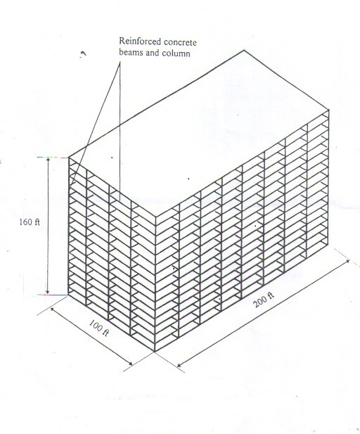Figure 1:Structural system of the 48.8m tall building

2.2.  Area of the study

 Wind speed data of Ikeja, Lagos state, Nigeria was used with reference to the wind speed map of Nigeria determined from40years of measurement at 10m height.

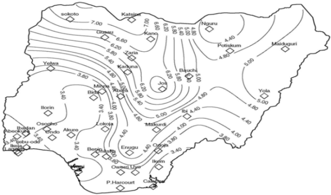Figure 2: Nigerian wind map in m/s determined from 40 years measurements at 10m height, obtained from Nigerian metrological department, oshodi, lagos state, Nigeria (NIMET).

3.       Analytical Procedure

From the wind speed map above it can be deduced that Lagos State (Ikeja) has a wind speed of 3.40m/s measured from a 10 meter height. Using [16], wind speed at subsequent height can be calculated with results, as follows:

The logarithm wind profile relationship is

Where  =wind speed at height, z is the building height,  is the friction velocity=0.3027m/s, k is the von Karman constant=0.41 and  is the roughness length=0.1m

Table 1: Wind speed as per log profile law

Storey height	Floor Height(m)	Wind velocity(m/s)
15th floor	48.77	4.569
14th floor	44.10	4.507
13th floor	40.95	4.440
12th floor	37.80	4.382
11th floor	34.65	4.317
10th floor	31.50	4.247
9th floor	28.35	4.169
8th floor	25.20	4.082
7th floor	22.05	3.984
6th floor	18.90	3.870
5th floor	15.75	3.735
4th floor	12.60	3.571
3rd floor	9.450	3.358
2nd floor	6.300	3.059
1st floor	3.150	2.547

The fundamental wind speed of the tall building 15^th floor = 4.569m/s

Now, the Design wind speed as per [15] can be calculated as

                      V_s= V_b S_a S_d S_s S_p                                      (2)

                      S_a=1+0.001 (3)

To determine the standard effective wind speed

                       V_e= V_s.S_b                                                                      (4)

Calculate the dynamic pressure

                       q_s=0.613V_e²                                                                (5)

To calculate the external wind pressure on the windward, leeward and sidewall of the high-rise building.

According to table 7, 8 and 9 of [15], C_pe for leeward wall and sidewall have negative values which accounts for the negative values of their wind pressures.

Where V_sis the site wind speed, V_b is the basic wind speed,V_e is standard effective wind speed, S_a is an altitude factor,  is the site altitude in meters,S_d is a direction factor,S_s is aseasonal factor,S_p is a probability factor,S_b is the roughness factor,q_s is the dynamic pressure, P_e stands for the wind pressure,C_a is the size effect factor for external pressure,C_pe is the external pressure coefficient for the building surface.

4.       CFD Analysis Procedure

4.1.  Computational Domain

Generally, the size of the entire computational domain depends on the targeted area and the boundary condition [9].

A key part of the modeling is the choice of the domain size and the positioning of the (single) high-rise building within that domain. Recent CFD studies have used [11] as a starting point in determining the domain size. The recommendation from [11] are as follows: the inlet, the lateral and top boundary are 5H away from the building where H is the building height, blockage ratio should exceed 3%[12] and the outlet should be positioned at least 15H behind the building.

The computational domain used for the study was given According to recommendations by [11], the inlet, the lateral and the top boundary away from the high-rise building model was 5H. while outflow boundary is 15H, leading to a blockage ratio of 1.8%. Where H represents the height of the building.

It is important to choose proper boundary condition since these decide to a large extent the solution in the computational domain [10]. Data generation used to describe the boundary conditions of the CFD study are presented in section 4-5, based on full scale measurements where relevant.

The governing equation for all fluid flow is the Navier Stokes Equation (7), (8), (9), (10)

The 2nd part of the equation is the viscous term, the 3^rd part is the pressure gradient and the 4^th part is the convective term

In order to describe the turbulent flow, the instantaneous term in equation (7), (8), (9),(10) is decomposed into its mean and fluctuating part as follows

                        U=U+uⁱ                                                                             (11)

                        V=V+vⁱ                                                                             (12)

                        W=W+wⁱ                                                                         (13)

                        P=P+pⁱ                                                                                (14)

Substituting equation (11), (12), (13), (14) into equation (7), (8), (9), (10), results to a time averaged solution to the Navier Stokes Equation for an incompressible fluid flow:

Where U, V, W are velocity vectors, P is pressure, ], ], ] from equation (15), (16) and (17) are referred to as Reynolds stresses because they are fluctuating component from the convective term of equation (8), (9) and (10)

Turbulence model is used to model the Reynolds stresses in order to close the RANS equation of fluid flow. It is an unfortunate fact that no single turbulence model is universally accepted as being superior for all classes of problem. The choice of turbulence model will depend on consideration such as the physics encompassed in the flow, the established practice for a specific class of problem and the level of accuracy required.

For this case study, RNG K- model by [17] was used for the modeling of turbulence because of its superior responsiveness to the effect of streamline curvature, vortices and rotations. Using this model, results into two addition equation (“k” and “ ”)

4.2.  RNG K  Turbulence quatity transport equation:

For  =   C^*_2e

Where C^*_2e =  , =  and S= (2S_ijSij)^1/2. k is the turbulence kinetic energy of the flow,  is the disspitation energy, =1.42, =1.68, = 0.0845, , .

4.3.   Inflow Boundary

At the inflow boundary layer, the mean velocity profile is usually obtained from the log profile corresponding to the upwind terrain via the roughness length Z_0.

For steady RANS simulation, the mean velocity profile and turbulence quantity are obtained based on the formula suggested by [18], in which the vertical profile for  stands for velocity, turbulence kinetic energy and dissipation energy respectively in the atmospheric boundary layer assuming a constant shear stress with height as follows:

4.4.   Outflow Boundary

At the downwind boundary, an outflow boundary was used with constant static pressure and boundary condition for  set to those of inlet. Backflow was not observed because the outlet boundary was sufficiently far away from the building.

4.5.   Wall Boundary

According to [19], within the computational domain, generally three different regions can be distinguished.

• The central region of the domain where the actual obstacle (building) are modeled explicitly with their geometrical shapes.
• The upstream and downstream region where the actual obstacles are modeled implicitly, i.e. their geometry is not included in the domain but their effect on the flow can be modeled in terms of roughness e.g., by means of wall functions applied to the bottom of the domain.

On the ground, a rough wall was specified to model the effect of the ground roughness. According to [19],

Where  is aerodynamic roughness length=0.1m, roughness constant ) =0.5. No slip boundary type was specified for the wall velocity

4.6.   Top Boundary

As also specified by [18], specific attention is needed for the boundary condition at the top of the domain, along the length of the top boundary, the values from the inlet profile of  at this height are imposed. ( , ). According to [19], the application of this particular type of top boundary condition is important because other top boundary condition (symmetry, slip, wall, etc) can themselves cause stream wise gradient in addition to those caused by wall function.

5.       Solver Setting

SIM-FLOW commercial CFD code was used to perform the simulation. The 3D steady RANS equation was solved. The simple algorithm was used for pressure-velocity coupling, pressure interpolation was second order and second- order discritizaton scheme were used for both the convective terms and the viscous terms of the governing equation for fluid flow.

6.         Results and Discussions

The turbulent nature of wind is a key parameter for high rise buildings and needs to be analyzed accurately in pre-construction and post-construction stages of the building.A body can be considered as an aerodynamic bluff when flow streamlines do not follow the surface of the body similar to the case of streamlined body but detach from it bearing regions of separated flow and wide trailing wake [6].

It is very important to understand flow patterns around buildings in order to validate the model results in wind simulation. As shown in figure 3 and 4, wind flows around the typical high-rise building with the boundary layer wind velocity profile. The CFD simulation was able to display regions of flow separation as well as wake of the bluff body. When wind flows around bluff bodies and comes across regions of adverse pressure gradients (positive pressure gradients), the flow separates and depending on the geometry of the bluff body forms series of recirculation flows at the downstream (leeward wall) usually referred to as wake as can be seen in figure 3 and 4 below. This wake accounts for the lower negative pressure (suction) experienced along that region.

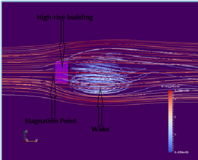Figure 3: Plan view showing flow separation and wake around the high-rise building

The average wind pressure obtained in CFD was compared to the design wind pressure prediction of [15].the author found out considerable disparity in regards to the wind pressure distribution. [15], assumes higher positive wind pressure at the top of the high-rise building with a value of 0.043kpa in cognizance to the ideology that pressure increases as velocity with height. Whereas, the CFD analysis shows that pressure distribution do not constantly follow that ideology. According to the CFD analysis, a value of 0.013kpa was calculated as the maximum pressure at the windward wall located in the 6^th floor as shown in table 2 but as we go higher up to the 10^th floor, this value is seen to decrease down to 0.012Kpa at the 11^th floor as can be seen in table 2.

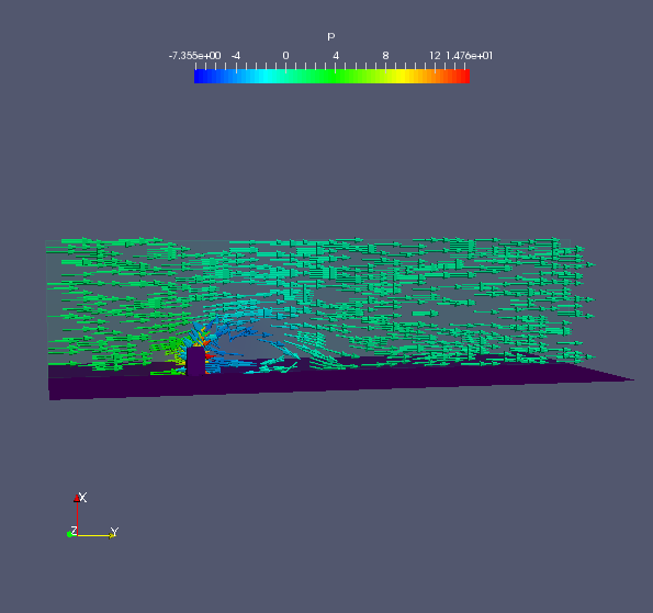Figure 4: symmetrical view of wind around the high-rise building

Table 2: windward pressure via CFD analysis

Floor	Height(m)	Wind P (kpa)
15th	48.768	-0.0256
14th	44.8	0.0798
13th	40.98	0.0100
12th	37.8	0.0112
11th	34.65	0.0122
10th	31.5	0.0130
9th	28.35	0.0135
8th	25.2	0.0136
7th	22.05	0.0134
6th	18.9	0.0130
5th	15.75	0.0124
4th	12.6	0.0119
3rd	9.45	0.0113
2nd	6.30	0.0109
1st	3.150	0.0108

Table 3: windward pressure via BS6399-2:1997

Floor	Height(m)	Wind P (kpa)
15th	48.768	0.04304
14th	44.8	0.04172
13th	40.98	0.04075
12th	37.8	0.03972
11th	34.65	0.03860
10th	31.5	0.03740
9th	28.35	0.03584
8th	25.2	0.03394
7th	22.05	0.03178
6th	18.9	0.02933
5th	15.75	0.02643
4th	12.6	0.02292
3rd	9.45	0.01844
2nd	6.30	0.01382
1st	3.150	0.009584

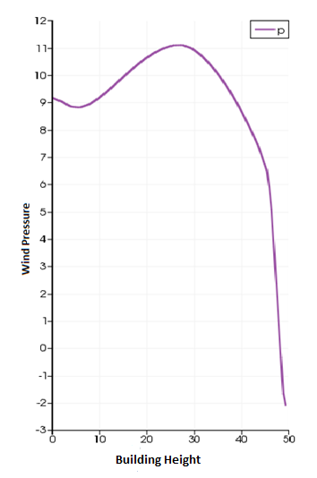Figure 5: windward pressure as per CFD analysis

Pressure coefficient is a dimensionless number which describes the relative pressure throughout a flow field in fluid dynamics. Wind pressure coefficients are generally estimated by assuming an incompressible fluid scenario and using the equation given below;

Where  is the pressure coefficient,  is pressure at location of interest,  static pressure,  is air density,  is the velocity at reference location.

Table 4: pressure and Cp value at windward wall via CFD analysis

Floor	Height(m)	Pressure(Kp)	Pressure(
1st	3.150	0.0108	0.8
2nd	6.300	0.0109	0.8
3rd	9.450	0.0113	0.8
4th	12.60	0.0119	0.9
5th	15.70	0.0124	0.9
6th	18.70	0.0130	1.0
7th	22.05	0.0134	1.0
8th	25.20	0.0136	1.0
9th	28.35	0.0135	1.0
10th	31.50	0.0130	1.0
11th	34.65	0.0122	0.9
12th	37.80	0.0112	0.8
13th	40.95	0.0100	0.7
14th	44.80	0.0798	0.6
15th	48.77	-0.0257	-0.2

The maximum pressure coefficient on the windward, leeward and sidewall of the high-rise building according to the CFD analysis are 1.0,-0.48 and -0.61 respectively. The of 1.0 observed at the windward wall of the high-rise building signifies stagnation point. Stagnation points are the point on the high-rise building where the local velocity (  is 0).

 

Table 5: Pressure and Cp value at leeward wall via CFD analysis

Floor	Height(m)	Pressure(Kp)	Pressure (
1st	3.150	-0.065	-0.50
2nd	6.300	-0.063	-0.49
3rd	9.450	-0.062	-0.48
4th	12.60	-0.061	-0.48
5th	15.70	-0.061	-0.48
6th	18.70	-0.016	-0.48
7th	22.05	-0.063	-0.49
8th	25.20`	-0.064	-0.50
9th	28.35	-0.066	-0.51
10th	31.50	-0.068	-0.52
11th	34.65	-0.069	-0.54
12th	37.80	-0.071	-0.55
13th	40.95	-0.072	-0.57
14th	44.80	-0.076	-0.59
15th	48.77	-0.081	-0.63

Table 6: Pressure and Cp value for sidewall via CFD analysis

Floor	Height(m)	Pressure(Kp)	Pressure (
1st	3.150	-0.088	-0.68
2nd	6.300	-0.089	-0.69
3rd	9.450	-0.091	-0.71
4th	12.60	-0.092	-0.72
5th	15.70	-0.092	-0.72
6th	18.70	-0.093	-0.72
7th	22.05	-0.094	-0.73
8th	25.20	-0.096	-0.75
9th	28.35	-0.097	-0.76
10th	31.50	-0.097	-0.76
11th	34.65	-0.096	-0.75
12th	37.80	-0.096	-0.75
13th	40.95	-0.095	-0.74
14th	44.80	-0.091	-0.71
15th	48.77	-0.079	-0.61

Table 7: Pressure and  value for windward wall as per BS6399-2:1997

Floor	Height(m)	Pressure(Kp)	Pressure (
1st	3.150	0.0096	0.600
2nd	6.300	0.0138	0.600
3rd	9.450	0.0184	0.665
4th	12.60	0.0229	0.732
5th	15.70	0.0264	0.772
6th	18.70	0.0293	0.799
7th	22.05	0.0318	0.818
8th	25.20	0.0339	0.833
9th	28.35	0.0358	0.844
10th	31.50	0.0374	0.850
11th	34.65	0.0386	0.850
12th	37.80	0.0397	0.850
13th	40.95	0.0407	0.850
14th	44.80	0.0417	0.850
15th	48.77	0.0430	0.850

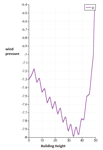Figure 6: maximum pressures on leeward and side wall

Table 7: Pressure and  value for Leeward wall as per BS6399-2:1997

Floor	Height(m)	Pressure(Kp)	Pressure (
1st	3.150	-0.0080	-0.5
2nd	6.300	-0.0115	-0.5
3rd	9.450	-0.0139	-0.5
4th	12.60	-0.0157	-0.5
5th	15.70	-0.0171	-0.5
6th	18.70	-0.0184	-0.5
7th	22.05	-0.0194	-0.5
8th	25.20	-0.0204	-0.5
9th	28.35	-0.0212	-0.5
10th	31.50	-0.0220	-0.5
11th	34.65	-0.0227	-0.5
12th	37.80	-0.0234	-0.5
13th	40.95	-0.0240	-0.5
14th	44.80	-0.0245	-0.5
15th	48.77	-0.0253	-0.5

Table 8: Pressure and  values for Sidewall A as per BS6399-2:1997

Floor	Height(m)	Pressure(Kp)	Pressure (
1st	3.150	-0.0216	-1.3
2nd	6.300	-0.0307	-1.3
3rd	9.450	-0.0370	-1.3
4th	12.60	-0.0417	-1.3
5th	15.70	-0.0455	-1.3
6th	18.70	-0.0487	-1.3
7th	22.05	-0.0516	-1.3
8th	25.20	-0.0540	-1.3
9th	28.35	-0.0562	-1.3
10th	31.50	-0.0582	-1.3
11th	34.65	-0.0599	-1.3
12th	37.80	-0.0617	-1.3
13th	40.95	-0.0632	-1.3
14th	44.80	-0.0646	-1.3
15th	48.77	-0.0666	-1.3

Table 9: Pressure and  value for Sidewall B as per BS6399-2:1997

Floor	Height(m)	Pressure(Kp)	Pressure (
1st	3.150	-0.0133	-0.8
2nd	6.300	-0.0189	-0.8
3rd	9.450	-0.0227	-0.8
4th	12.60	-0.0257	-0.8
5th	15.70	-0.0280	-0.8
6th	18.70	-0.0299	-0.8
7th	22.05	-0.0317	-0.8
8th	25.20	-0.0332	-0.8
9th	28.35	-0.0346	-0.8
10th	31.50	-0.0358	-0.8
11th	34.65	-0.0369	-0.8
12th	37.80	-0.0379	-0.8
13th	40.95	-0.0389	-0.8
14th	44.80	-0.0398	-0.8
15th	48.77	-0.0410	-0.8

According to Bernoulli’s equation, static pressure is at its maximum value at stagnation point. This static pressure is called stagnation pressure. As can be seen in table 4, from the 30^th -50^th floor where  is 1.0 recorded the highest wind pressure on the windward wall.

Whereas, [15], prescribed the pressure coefficient of 0.85,-0.5, and -1.3 as maximum value at the windward, leeward and sidewall of the high-rise building respectively.

7.         Conclusion

The wind pressure at different levels of the high-rise building obtained from CFD simulation for the 48.767m high-rise building were compared to the predictions given by [15]. More so, the limitations of the three methods in calculating wind loads on high-rise buildings (BS6399-2:1997, wind tunnel testing and CFD) were discussed.

The researcher also statedthat with strict adherence to the CFD best practice guidelines for wind around buildings stipulated in [10], [12], [13], CFD can serve as an alternative approach to the costly and time-consuming wind tunnel testing in predicting with considerable accuracy wind behavior around high-rise buildings both in the preliminary as well as final design stage of a project constructions. Also, result of the CFD analysis showed that the wind pressures obtained are usually lower than those predicted by [15] which can result in greater economy in the structural framing.

However, more experimental work is required to validate the CFD analysis. This work will take place at Nnamdi Azikiwe University awka, Nigeria.

1. M.Overend, K.Zammit; “wind loading on cladding and glazed facades”internatonal symposium on the application of architectural glass, ISSAG 2006.http//www.Isaag.com
2. Roshka, “perspectives on the bluff body aerodynamics” Journal of wind engineering and industrial aerodynamics, 41, 79-100(1993
3. K.bernard, “prediction of wind loads on tall building” PHD thesis University of western Ontini, (1993).
4. K.Nguyen “A study of aerodynamic wind loads on tall building using wind tunnel tests and numerical simulation” PHD thesis University of Melbourne
5. D.Kwon & A. Kareem, “Comparative study of major international wind codes and standards for wind effects on tall buildings” Engineering structures, vol.51, pp.23-35
6. D.Mohotti,P.Mendis,T.Ngo, “Application of computational fluid dynamics(CFD) in predicting the wind loads on tall buildings-A case study”.ACMSM23,Byron Bay Australia,(2014).
7. H.Montezeri, B.Blocken, “CFD Simulation of wind induced pressure coefficients in buildings with and without Balconies.
8. H.Versteeg, W.Malalasekera. “An introduction to computational fluid dynamcs: The finite volume method” England: Pearson education ltd
9. D.kim. “The application of CFD to building analysis and design: A combined approach of an immersive case study and wind tunnel testing”. PHD thesis, Virginia polytechnic institute and state university. USA
10. J.Franke, A.Hellsten, H.Schlunzen, B.Carrissimo,(2007) “best practice guidelines for the CFD simulation of flows n urban environment”. COST 732: quality assurance and improvement of micro scale meteorological models. Cost office Brussel, ISBN 3-00-018312-4
11. J.Franke,C.Hirsch,A.Jensen,H.Krus,M.Schatzmann,P.Westbury,S.Miles,J.Wisse,N.Wright,(2004) “Recommendations on the use of CFD in wind engineering”, COST ActionC14:Impact of Wind and storm on city life and Built Environment,von karman Instute for Fluid Dynamics.
12. Y.Tominaga,A.Mochida,R.Yoshie,H.Kataoka,T.Nozu,M.Yoshikara,T.Shirasawa,(2008).Aij guidelines around buildings .Journal of wind engineering and industrial Aerodynamics,96(10-11),1749-1761.ISSN 0167-6105,http://dx.doi.org/10.1016/j.jweia.2008.02.058
13. M.Casey, T.Wintergersk, “Best practice guidelines, ERCOFTAC special interest group on quality and trust in industrial CFD.ERCOFTAC, Brussels.
14. E.Vafaeihosseini, A.Saghels, R.Kumar, “Computational fluid dynamics approach for wind analysis of high-rise buildings: Report: 111T/TR/2013/1,center for earthquake engineering, international institute of information technology,Hyderabad,India.
15. BS6399-2:1997.Loading for buildings-part 2: code of practice for wind loads BSI
16. Online Available: http://en.m.wikipedia.org/wiki/log_wind_profile.
17. V.Yakhot,S.Orszag,S.Thangam,T.Gatski,C.Speziale,(1992) “Development of turbulence model for shear flows by a double expansion technique” physics of fluids A,Vol.4,No.7,pp1510-1520
18. P.Richards & R.Hosey, “Appropriate boundary conditions for computational wind engineering model usng the K-e model”, J.wind eng.ind.aerod, 46-47,145-153
19. B.Blocken, T.Stathopoulos, J.Carmeliet, “CFD simulation of the atmospheric boundary layer: wall function problems”atmos.enviro, 41(2), 228-252.

(Click to view)

(Click to view)