1. Introduction

Nowadays, turbines have become a very important engineering development with several applications in almost all markets not only the aviation industry but also from oil and fuel industry to daily commuting applications as mass transportation.

There are several types of turbines; however this article will be centered in gas turbines. A gas turbine operates within the principle the Joule – Brayton cycle where compressed air is mixed with fuel, and afterwards burned under constant pressure conditions [Weston, 1992]. A gas turbine energy plant is an internal combustion system that converts chemical energy released from the burned fuel into heat energy, which converts to mechanical and/or electrical energy at the output of the process [1].

A simple gas turbine power plant consists of three main components: a compressor, a combustor, & a gas turbine. The resulting high pressure gas is expanded through the turbine to perform work output often used to drive a shaft connected to a mechanical arrangement in order to produce the required form of energy (mechanical/electrical).

A gas turbine, commonly called, combustion turbine, consists of an upstream rotating compressor coupled to a downstream turbine with a combustion chamber in between. The increasing usage & applications of gas turbines drive the necessity to design more complex dynamic systems. For such enterprise, the necessity, to understand turbo machinery behavior & deep knowledge on how to control them, has grown exponentially [2].

1.1.  Mathematical models of Gas Turbines.

Diving into mathematical models of gas turbines; one of the mostly used is the Rowen’s model which is a simplified mathematical representation of four gas turbines covering a horsepower range from 26,000 HP to 108,000 HP. The model incorporates, both, the control and fuel system characteristics as well as those relative to the turbo machinery. This model is suitable for a wide range of ambient temperatures, and the influence of axial flow compressor variable inlet guide vanes is included in the models as appropriate to the actual machinery configuration. The Rowen’s Model is one of the vastly used mathematical models in turbo machinery applications as it also incorporates control system logic [3].

Other example of mathematical models is led by the Department of Mechanical and Process Engineering in the ETH based in Zurich which has been working in smart controlled gas turbines to obtain fuel efficient-reliable operation [4].

A control-oriented model is necessary for the purpose of modeling and fault detection. An oriented model defines the input-output behavior of the micro gas turbine system with reasonable precision at low computational complexity. It is designed to include explicitly all relevant transient effects and is represented by a set of nonlinear ordinary differential equations, which are derived from physical first principles [5].

1.2.  Operation of the Gas Turbine.

The basic operation of the gas turbine is similar to the steam power plant except that air is used instead of water. Fresh atmospheric air flows through a compressor that brings it to higher pressure. Energy is then added by spraying fuel into the air and igniting it so the combustion generates a high-temperature flow. This high-temperature with high-pressure gas enters a turbine, where it expands down to the exhaust pressure, producing a shaft work output in the process.

The turbine shaft work is used to drive the compressor and other devices such as an electric generator that may be coupled to the shaft. The energy that is not used for shaft work comes out in the exhaust gases, so these have either a high temperature or a high velocity. The purpose of the gas turbine determines the design so that the most desirable energy form is maximized. Gas turbines are used to power aircraft, trains, ships, electrical generators, or even tanks [6, 7].

In an ideal gas turbine, gases undergo three thermodynamic processes: an isentropic compression, an isobaric (constant pressure) combustion and an isentropic expansion. Together, these make up the Brayton cycle. That is shown below:

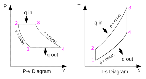Figure 1. The Brayton cycle [8].

In a practical gas turbine, mechanical energy is irreversibly transformed into heat when gases are compressed (in either a centrifugal or axial compressor), due to internal friction and turbulence. Passage through the combustion chamber, where heat is added and the specific volume of the gases increases is accompanied by a slight loss in pressure. During expansion the stator and rotor blades of the turbine, irreversible energy transformation, once again, occurs.

2.       Main variables in the system.

2.1.  Main sections of a Gas Turbine.

The combustion (gas) turbines are being installed in many of today’s natural-gas-fueled power plants and they are complex machines, but they basically involve three main sections.

Beginning with the air intake design; this drag air into the compressor which pressurizes it and feeds it to the combustion chamber inside the engine at speeds of hundreds of miles per hour. Then, the combustion system typically made up of a ring of fuel injectors that inject a steady stream of fuel into combustion chambers where it mixes with the air supplied. The mixture is then burned at temperatures of more than 2000 degrees F. The combustion produces a high temperature, high pressure gas stream that enters and expands through the turbine section.

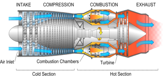Figure 2. Main sections in a gas turbine [9].

The turbine, finally, is an intricate array of alternate stationary and rotating aerofoil-section blades. As hot combustion gas expands through the turbine, it spins the rotating blades. The rotating blades perform a dual function: they drive the compressor to draw more pressurized air into the combustion section, and they spin a generator to produce electricity [10].

2.2.  Main variables from the thermodynamic process.

The main stage variables are defined based upon the independent states within the thermodynamic process during the Brayton cycle. As it is shown in the next image, there are 4 main states during the process in which all the variables involved have a different behaviour in specific points through the cycle but these does not mean that the variables will remain static throughout the entire process.  Refer to figure 5 to understand the different stages within the cycle.

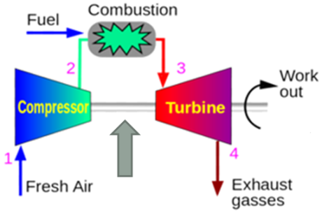Figure 3. Main sections of a Gas Turbine [11].

The main variables in a thermodynamic process are: density, pressure, temperature and fluid velocity.

The Joule-Brayton Cycle illustrates the basic Gas Turbine stages during the transformation process of fluid energy into rotatory work; in each step there are specific conditions (isentropic compression & expansion as well as isobaric combustion and cooling) that must need to be taken into account during the mathematical modelling definition [11].

3.       Mathematical model

The mathematical model was developed using the physics conservation laws such as the mass conservation, the linear momentum conservation, the ideal gases equation and the energy conservation.

3.1.  Continuity equation.

The continuity equation is governed by the principle that mass is neither created nor destroyed, just transformed. This principle is one of the foundations in the study of fluids movement. This concept is defined by differential and integral equations. Consider an arbitrary control volume in a flux. By the principle of conservation of mass, the sum of the mass variation rate from inside the volume and the mass that travels to the surface of the volume is zero. Figure 6 describes the mass conservation through the control volume:

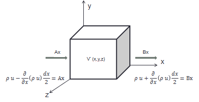Figure 4. Control volume for the mass conservation.

Where Ax is the mass flux that enters the system and Bx is the mass flux that is leaving the system through the x axis. For the value of Ax and Bx it is necessary to use a Taylor series expansion and the equation is the next one:

The change rate of the accumulated mass flow is given by the next equation:

Finally, by applying the same analysis in all axes and gathering the terms in equation (2), the result is the continuity equation:

3.2.  Cauchy equation.

The previous analysis using CV for the mass conservation is also used for the linear momentum conservation. It is necessary to apply the Newton’s second law to a differential fluid element. This also holds that the sum of the forces on a particle is equal to the rate of change of its linear momentum.

The CV that holds the linear momentum conservation is the same that in the previous analyses:

Where Ax is the linear conservation that enters the system and Bx is the linear conservation that is leaving the system through the x axis. Also it is necessary to use a Taylor series expansion. The equation that holds this is the next one:

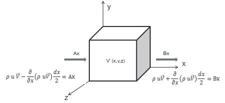Figure 5. Control volume for the linear momentum conservation.

The change rate of the accumulated linear momentum is given by the next equation:

By applying the same analysis as in the continuity equation and gathering the terms in equation (5), and equalling to the surface and body forces, the resulting is the Cauchy equation:

And finally for the right hand side of the equation (6), it holds that the body forces are just the gravity and the surface will be manage as an input, so [12,13,14]:

3.3.  Energy differential equation.

The first law of thermodynamics states the conservation of energy. Considering a system, that changes in the power expressed by the sum of the input energy as heat and work. The power system comprises the internal energy and kinetic energy. The next figure represents the control volume of the conservation of energy in the system:

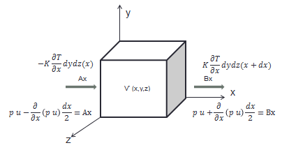Figure 6. Control volume for the energy conservation.

Where Ax is the amount of heat and works that enters and Bx is the amount of heat and work that comes out analyzed only on the x-axis:

And analysing the relations in the three axes of the quantity of fluid that occupies in the element infinitesimal generates the equation.

Given the equation of the first law of thermodynamics, the material derivative of the energy of the system is expressed as follows:

The next equation is the equation that involves the temperature in the system and by adding some terms relate of the shear forces expressed everything in a vector form is the equation well known as the energy balanced equation [12,15,16]:

3.4.  State differential equation of ideal gases.

The ideal gas law is the equation of state of a hypothetical ideal gas. It is a good approximation of the behavior of many gases under many conditions, although it has several limitations.

The next images represent the curve lines of the relationship between pressure (on the vertical, y-axis) and volume (on the horizontal, x-axis) for an ideal gas at different temperatures: lines that are farther away from the origin represent higher temperatures.

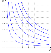Figure 7. Graph of isotherms ideal gases [17].

The ideal gas law is often written as :

{\displaystyle PV=nRT}Where:

• {\displaystyle P} is the pressure of the gas,
• V{\displaystyle V} is the volume of the gas,
• {\displaystyle n}n is the amount of substance of gas (in moles),
• {\displaystyle R}R is the ideal, or universal, gas constant, equal to the product of the Boltzmann constant and the Avogadro constant,
• {\displaystyle T}T is the absolute temperature of the gas.

The state of an amount of gas is determined by its pressure, volume, and temperature. Therefore, an alternative form of the ideal gas law may be useful. The chemical amount (n) (in moles) is equal to the total mass of the gas (m) (in grams) divided by the molar mass (M) (in grams per mole):

By substituting the last equation in equation number (12):

Subsequently introducing density ρ = m/V, we get:

Defining the specific gas constant R _specific(r) as the ratio R/M [12, 17]:

It is common, especially in engineering applications, to represent the specific gas constant by the symbol R. In such cases, the universal gas constant is usually given a different symbol such as to distinguish it. As establish pressure, density and temperature as variables, it is possible to derivate in respect of time and it obtains the next equation:

The equation (17) is the last one in order to describe a gas turbine behaves by differential equation.

3.5.  Mathematical modelling simplifications.

The next step is to express all derivate with respect of space in derivate with respect of time using the chain rule.

4.       Simulations.

The simulations results are plotted in 3 different steps, the first part represents the compressor, in which the main variable to follow is density; also temperature and pressure are plotted. Then the second step is the combustor, here the main variable to follow is the temperature but also the variable of density is plotted, just remembering that the combustion is an isobaric process, in other words, the pressure doesn’t suffer a significant change. Finally and control objective, the rotor; in here, it is necessary to keep a set point of velocity, because it is where all the work and main subsystems that the gas turbine will feed are connected. The next image is the Joule – Brayton cycle that represents the 3 main steps that just were described.

The first curve is the adiabatic compression; the second curve the isobaric combustion and finally the adiabatic expansion.

As explained during compression, the main variable that to be controlled is the density; Figure 11 represents  the hatch that allows the amount of air to pass while opened at 90% of its capacity thus generating a density approximately of 50 Kg/m^3.

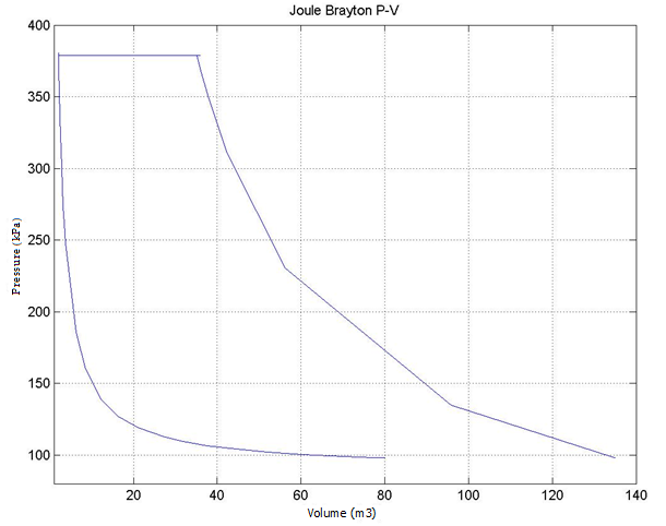Figure 8. Graph of isotherms ideal gases.

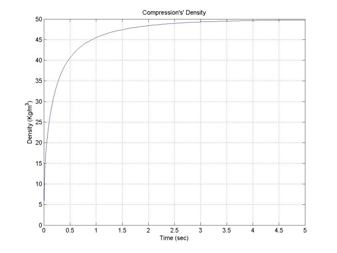Figure 9. Graph of density during compression.

Also the pressures temperature were plotted as seen on figure 10.

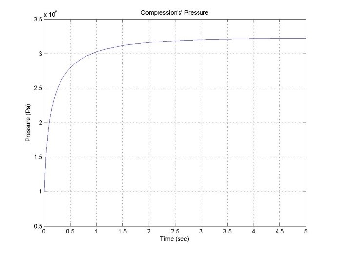Figure 10. Graph of pressure during compression.

The hatch opened at 90% of its capacity generating a pressure of 380 KPa approximately. The systems needs a certain fluid velocity to start working, for that reason the hatch it is opened proportionally during the first 15 seconds until the fluid velocity reached a speed of 80 m/s. Then the hatch is opened in one shot until 90% of it capacity.

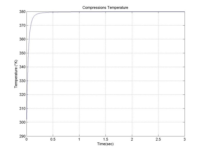Figure 11. Graph of temperature during compression.

The temperature reached during compression was 380°K approximately.

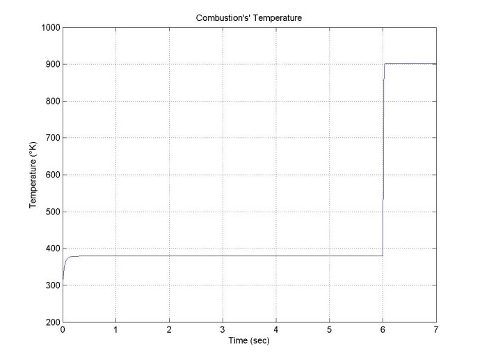Figure 12. Graph of temperature during combustion.

The highest temperature reached throughout all operating cycle was during combustion phase while opening the fuel hatch at 90% of its capacity as the main variable during this stage is temperature as combustion is done ay isobaric conditions so while the pressure stayed the same, the final temperature reached was 900°K approximately.

The objective of a gas turbine control logic is to be able to vary the rotor speed as needed at the precise timing. The next image shows the rotor behaviour through the cycle;, it splits into two different phases; first during compression and finally during combustion.

The last figure shows the final rotor velocity was 650 rev / seconds when the hatch of the air and fuel were opened at 90%.

5.       Future work

5.1.  Algorithm control in the system.

Advanced controlled systems based in mathematical modeling can sustain the next development steps as it increases the deep knowledge of what is happening from a complete system vision criteria and guarantees the results that are required, as it gives complete control of the rotor’s movement ,the speed that is required, the pressure inside the compressor and finally the temperature of the combustion chamber to work along with an inter-cooling system at the precise timing that is needed so the output of the cycle is within the expected range of efficiency and performance [18].

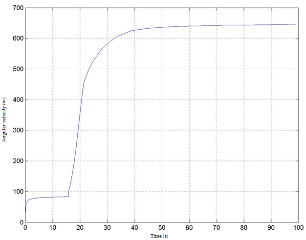Figure 13. Graph of the rotor velocity during compression and combustion.

For the implementation of this idea, new combustor and blade designs will be required to allow appropriate heat exchange between cold and hot fluids, ensuring high integrity and risk mitigation of the structural components as well as health and safety conditions respectively. New manufacturing techniques for these complex geometries will be required that can enhance mass transfer during the internal cooling cycle [19].

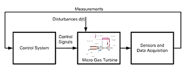Figure 14. Model-based and control-oriented diagnosis of a micro gas turbine [20].

6.       Conclusions

The complexity of the systems and the effective applications of gas turbines drive the need to develop highly complex mathematical models with a high accuracy in order to precisely control the turbine dynamics in order to exceed efficiency and performance balance. If correctly applied, it can be ensured that all the variables from the system cycle are going to be within the working limits conditions that the turbine would demands.  The model developed is based in the three main systems particular to the turbine: compressor of the fluid, rotor shaft and combustion chamber.

Finally, advanced controlled systems based in mathematical modeling increase the reliability of what is happening in the complete system giving a holistic view and guarantee the results that are required with an optimal efficiency.

1. Ekstrom, T. E. and Garrison, P. E., 1991, “Large Gas Turbines for Mechanical Drive Applications”, GER-3701, GE Company, Schenectady, NY, August 1991.
2. Rowen, W. I., 1983, “Simplified Mathematical Representations of Heavy Duty Gas Turbines”, ASME Paper 83-GT-63 and ASME Journal of Engineering for Power, October 1983, Page 865.
3. Simpson, C. Aalburg, M. B. Schmitz, R. Pannekeet, V. Michelassi, F. Larisch, “Application of Flow Control in a Novel Sector Test Rig”, Journal of Turbomachinery, 136(4), 041002 , Sep 26, 2013, TURBO-12-1249.
4. M. Sunar, S. S. Rao, “Recent Advances in Sensing and Control of Flexible Structures Via Piezoelectric Materials Technology”, Applied Mechanics Reviews, Vol.52.
5. J. Bordeneuve-Guibe, C. Vaucoret, “Robust multivariable predictive control: an application to an industrial test stand”, Control Systems IEEE, Vol. 21, Issue 2.
6. Ozsoy, A. Duyar, ; R. Kazan, R. Kilic, “Power turbine speed control of the GE T700 engine using the zero steady-state self-tuning regulator”, Intelligent Engineering Systems, 1997. INES ’97. Proceedings, 1997 IEEE International Conference on.
7. Zohuri, Brahman. “Gas Turbine Working Principles”, Combined Cycle Driven Efficiency for Next Generation Nuclear Power Plants, 2015.
8. Online: https://en.wikipedia.org/wiki/Brayton_cycle.
9. Online: http://cset.mnsu.edu/engagethermo/componentsgasturbine.html
10. Chacartegui, R., Sánchez, D., Muñoz, A., & Sánchez, T. (2011). Real time simulation of medium size gas turbines. Energy Conversion and Management. Modeling of off-design multistage turbine pressures by Stodola’s ellipse. Energy Incorporated, PEPSI user’s group meeting. Richmond, Virginia: Bechtel Power Corporation.
11. https://wn.com/gasturbine/wikipedia
12. Dixon, S. L. (1998). Fluid Mechanics and Thermodynamics of Turbomachinery, Fourth edition. Woburn, MA, USA: Butterworth-Heinemann.
13. P. Chiesa, E. Macchi, “A Thermodynamic Analysis of Different Options to Break 60% Electric Efficiency in Combined Cycle Power Plants”, ASME Turbo Expo 2002: Power for Land, Sea, and Air, Vol. 1: Turbo Expo 2002, ASME, GT2002-30663, pp. 987- 1002.
14. Online: https://www.boundless.com/physics/textbooks/boundless-physics-textbook/temperature-and-kinetic-theory-12/ideal-gas-law-104.
15. B. Facchini, L. Innocenti, E. Carnevale, “Evaluation and Comparison of Different Blade Cooling Solutions to Improve Cooling Efficiency and Gas Turbine Performances”, ASME Turbo Expo 2001: Power for Land, Sea, and Air, Vol.3: Heat Transfer; Electric Power; Industrial and Cogeneration, 2001-GT- 0571, pp. V003T02A025.
16. G. Richards, Williams M., and Casleton K. “Novel cycles: oxy-combustion turbine cycle systems”, Combined cycle systems for near-zero emission power generation, 2012.
17. Online: https://en.wikipedia.org/wiki/Idealgas.
18. L. Chi-Huang, T. Ching-Chih, “Adaptive Predictive Control With Recurrent Neural Network for Industrial Processes: An Application to Temperature Control of a Variable-Frequency Oil-Cooling Machine, Industrial Electronics IEEE Transactions on, 04/2008; 55(3):1366 – 1375.
19. García Nieto, Paulino, Esperanza García-Gonzalo, Antonio Bernardo Sánchez, and Marta Menéndez Fernández. “A New Predictive Model Based on the ABC Optimized Multivariate Adaptive Regression Splines [24] Approach for Predicting the Remaining Useful Life in Aircraft Engines”, Energies, 2016.
20. D.W. Clarke, “Application of generalized predictive control to industrial processes”, Control Systems Magazine IEEE, Vol. 8, Issue.

(Click to view)

(Click to view)