1          Introduction

A Boolean Satisfiability (abbreviated as SAT) problem involves a boolean formula F consisting of a set of boolean variables x₁,x₂,…..x_n. The formula F is in conjunctive normal form(CNF) and it is a conjunction of m clauses c₁,c₂,…..c_m. A clause is a disjunction of one or more literals, where a literal is a variable x_i or its negation. A formula F is satisfiable if there is a truth assignment to its variables satisfying every clause of the formula, otherwise the formula is unsatisfiable. The goal is to determine an assignment for every variable x satisfying all clauses.

The class k-SAT contains all SAT instances where each clause contains upto k literals. While 2-SAT is solvable in polynomial time, k-SAT is NP-complete for k>=3 . The SATs have many practical applications e.g. in planning, in circuit design, in spinglass model,in molecular biology and especially many applications and research on the 3-SAT is reported.

Some say that if we have an algorithm to solve k-SAT problem in polynomial time then cooking the food would become as easy as eating it. Speculations have been also there that a polynomial time algorithm might disapprove 2nd law of thermodynamics or can even find the god!

There are two approaches which are generally used to solve the SAT problem. The first one is local optimization or local search and the other one is genetic or evolutionary framework. The local search optimization technique is to assign some truth values to variables until we do not get a conflict[1]. After getting a conflict either the algorithm starts again or backtracks to change the value of the variable which is responsible for the conflict. So this approach uses backtracking hence time-complexity wise is not suitable (especially for large instances containing hundreds and thousands of variables). The most common algorithms in local search optimizations are GSAT(Greedy SAT)[2] and WalkSAT.

The other approach is to come up with an evolutionary algorithm[3, 4] for solving the SAT problem. They are admittedly quite fast than the traditional local search methods. However, if a given SAT instance is satisfiable but the program fails to come up with a satisfying instance within the limited time period, then it would wrongly judge the given instance as unsatisfiable. Hence it is an incomplete algorithm.

These genetic approaches involve many other factors such as crossover, mutation, parent selection and the most important factor, the fitness function. Till date we have many approaches proposed so far. For example, the SAWEA , the RFEA and RFEA2+ are based on adaptive fitness functions and use problemspecific mutation operators[5]. The FlipGA and ASAP use the MAXSAT fitness function and a local search procedure. The MAXSAT fitness value is equivalent to the number of satisfied clauses.

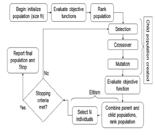Figure 1: Basic flow chart of Genetic Algorithm design

2          Proposed Algorithm

Our algorithm combines the power of local search along with the Genetic Algorithm.

The Trivial Case:

We first check if there isnt any clause present in our formula such that all of its constituent literals are positive (negative). If this is the case, then we can immediately find a solution by assigning False (True) to all the variables.

Trivial()

• CountAllPos = No. of clauses with all constituent literals positive.
• CountAllNeg = No. of clauses with all constituent literals negative.
• If (CountAllPos == 0)• Assign False to every variable.
• Else if(CountAllNeg == 0)• Assign True to every variable.
• End if.
• Continue with the main algorithm.

We then eliminate all the unit literals (if present) and the pure literals (if present).

• Unit Literal Rule: If a literal appears as the sin-gle constituent of a clause in the formula, then we can safely delete all those clauses containing that literal. We also then remove the negated form of this literal from every clause in the formula where it appears.
• Pure Literal Rule: If a variable appears only init’s positive(negated) form in the whole formula, then all the clauses containing that variable can be safely deleted.

Although the benchmarks problems that we used for our experiments[6] were carefully designed not to allow this technique, however, in any random SAT instance[7] those two techniques hold good and reduce the search space to a great extent[Table 1].

Our Algorithm

1. Try the Trivial Case.
2. If solution not found yet, Eliminate Unit Literals.
3. If solution not found yet, Eliminate Pure Literals.
4. If solution not found yet, implement GeneticAlgorithm.

Every chromosome in our algorithm is represented as a bit-string of length n , where n is the no of variables present in the formula.

Genetic Algorithm()

• TOTAL GEN = 1
• CURRENT GEN = 1
• MAX FITNESS = 0
• Generate random population of size POP SIZE
• Assign fitness values to every individual of thepopulation
• For each individual a:
• If fitness(a) equals NO OF CLAUSES:
• Print Satisfiable
• Exit
• Else if fitness(a) is greater than MAX FITNESS:
• LAST GEN = CURRENT GEN
• MAX FITNESS = fitness(a)
• End if
• Sort the population by their fitness values andtransfer (ELITISM RATE * POP SIZE) top most individuals (the ones with the higher fitness) to the next generation

• To fill up the remaining places for the new gen-eration do the following:
• Select two fittest individuals from the current generation using Roulette-Wheel selection technique
• Apply Crossover between them. (dependent on the CROSSOVER RATE)
• Apply Mutation between them. (dependent on the MUTATION RATE)
• Transfer the new individuals to the next generation
• Repeat till all places for the new generation are filled
• Increment CURRENT GEN
• If (CURRENT GEN – LAST GEN) > LIMIT:
• TOTAL GEN=TOTAL GEN+CURRENT GEN
• If TOTAL GEN > MAX GEN:
• Print Not Satisfiable
• Exit
• Else goto Step 2
• End if
• Else goto Step 5
• End if

2.1       Different Parameters

Parameters used in our algorithm:

1. MAX GEN : Maximum no of generations allowed for our program to run.
2. ELITISM RATE : The fraction of the total no of individuals in our current generation that would be transferred to the next generation.
3. CROSSOVER RATE : Determines the probability that two selected individuals would perform crossover.
4. MUTATION RATE : Determines the probability that the concerned individual would undergo mutation.
5. POP SIZE : The total no of individuals in any generation.
6. LIMIT : Specifies a threshold, if no improvement occurs for a given span of generations (specified by LIMIT), then a new fresh random population is generated.

The various crossover functions used:

1. Single Point Crossover : We select a pivot point(randomly) ranging between 0 to length of the chromosome and then exchange the substring from the pivot till the end of the string between the two chromosomes.
2. Two Point Crossover: We select two pivot points(randomly) ranging between 0 to length of the chromosome and then exchange the substring defined within those two points between the chromosomes.
3. Uniform Crossover: We exchange every alternate bit between the two chromosomes.
4. Greedy Crossover: This is similar to the SinglePoint Crossover, however we choose the pivot point in a greedy fashion.

As a precomputation step, we first build a table of size 2*no. of variables (as we can have this many different literals possible) and store in it the no of clauses satisfied by the corresponding literal.

So, Table[a] would store the no of clauses that the literal a would satisfy independently. We define prefix sum array ’Pre’ and suffix sum array ’Suff’ for a given chromosome C = x₁x₂x₃x₄x_n as follows :

Pre[i] = Table[x₁] + Table[x₂] + …..Table[x_i]

Suff[i] = Table[x_i+1] + Table[x_i+2] +…..Table[x_n]

Hence given a chromosome pair C1 and C2, we compute their prefix sum arrays Pre1, Pre2 and their suffix sum arrays Suff1 and Suff2 as described above.

We choose the pivot point by the following formula,

Pivot = index for which max(Pre1[index] +

Suff2[index], Pre2[index] + Suff1[index]) is maximum for all index from [0…..length – 1] , where length is the length of the chromosome.

5. Fixed Length Crossover: We want to find out the optimal length of the crossover (the length of the substring to be swapped between the two chromosomes). So we experiment with various lengths. For a given length l, we maintain a sliding window of length l and then shift the window from left to right , and we finally swap that substring of length l (contained within that window) such that the resulting individual has the maximum fitness . We define r = Ratio of Crossover Length to Chromosome length. i.e. r = l/n. The results are displayed in Fig. 6 and

Fig. 7.

The various mutation functions used:

1. Single bit flip – Flip a single bit (chosen randomly).
2. Multiple bit flip – Flip multiple bits (chosen randomly).
3. Single bit greedy – Flip a single bit which increases the fitness value for that individual.
4. Single bit max greedy – Flip that single bit whichincreases the fitness value for that individual to the highest as compared to flipping any other bit.

5. Multi bit greedy – Keep flipping bits (from leftto right) which increases the fitness of that individual. (only a single left to right iteration).
6. FlipGA[8] – Keep flipping bits from left to rightwhich increase the fitness of that individual. Once the right end is reached, again start from the left end until no more flipping is possible.

Mutation functions 1 and 2 are dependent on MUTATION RATE. The rest aren’t (due to forced mutation).

3          Experiments

POP SIZE = 100

CROSSOVERRATE = 0.7

MUTATIONRATE (does not matter as we used Multi bit Greedy)

LIMIT = 50

MAX GEN = 500

The results were pleasant for instances with lesser no. of variables, however with large test cases (involving more than 80 variables) the success ratio could barely make it to 60%.

We then increased our POP SIZE to 500, which improved the success rate but made our program to run extremely slow! This is because the mutation function that we were using (Multi bit greedy) was costly enough.

So we finally resorted to introduce the concept of elitism in our algorithm. We experimented with various elitism rates and found out that a 60-70 % of elitism yields best results on an average (based on runtime and success ratio).

So the final parameters for our experiments were-

1. POP SIZE = 500
2. CROSSOVER RATE = 1
3. MUTATION RATE (does not matter as we used Multi bit Greedy)
4. LIMIT = 40
5. MAX GEN = 200
6. ELITISM RATE = 0.7

• Since we were using a high elitism rate so mostof the population went on to the next generation without being mutated, so the costly mutation function needed to be used for a comparatively small part of the population, which improved the runtime.
• As we were anyway transferring 70% of the bestindividuals (the ones with the maximum fitness) from the current generation to the next generation, so we would like to have the remaining 30% of the new generation to be fulfilled by completely new individuals. Hence we set the CROSSOVER RATE to 1 to increase the chances of getting new individuals drastically.

4          Results

As evident from Figure 2 and Figure 3 our algorithm performed quite well till test cases containing 100 variables. This had been a significant improvement over what we had achieved earlier. We also noticed that the success rate could be further increased by increasing the MAX GEN (increasing the POP SIZE increases the runtime drastically, so we should not increase it much), however at the cost of increased runtime.

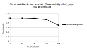Figure 2: Success Rates

Variables

Clauses

Clauses Reduced

Time(in sec)

5	20	0	0.031
50	100	10	0.054
100	200	12	0.332
25	100	0	0.069
250	1000	25	101.298
256	6336	0	107.626

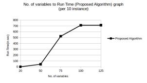Figure 3: Run Times

Table 1: Table for Random Instances(all satisfiable)

4.1        Comparative Analysis

4.1.1        Different Crossovers

Success Rate: Clearly from Figure 4 we see that the Two point crossover performed quite well in our experiments. The Single point crossover and Greedy crossover overlap in some areas and are comparable to each other. It remains to see how they perform for instances with a very large no of variables.

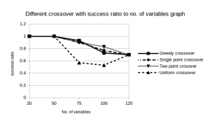Figure 4: Success Rates of Different Crossover functions

However,a striking fact is that the uniform crossover yielded quite unsatisfactory results. We were flummoxed with its results and so to crosscheck our data we ran the program again but still the results were the same. Looks like this crossover is definitely not a choice for the Boolean Satisfiability problem. Our implementation of uniform crossover was though, nave. It just flipped the alternating bits. It remains to see if introducing probabilistic methods to choose which bits to flip can increase the performance of this algorithm.

Runtime: Figure 5 suggests that Single point crossover and Two point crossover are the fastest (and yield good success rates as well ). However, the Greedy Crossover has to perform a lot of precomputations and hence it has a larger runtime. The runtime of the Uniform Crossover doesnt really matter as it yielded a quite poor success rate.

Figure 5: Run Times of Different Crossover functions

Fixed-length crossover:

We know that during the crossover phase there is an exchange of genes between the chromosomes (or namely, in our algorithm it is represented as an exchange of a substring between the two chromosomes, which themselves are represented as bit strings). What should be the ideal length of the substring to be exchanged? We tried to address this problem by conducting various experiments. We assumed that this ideal length would be a function of the no of variables present in the problem statement.

Let l be the Crossover length , i.e. the length of the substring to be exchanged between the chromosomes.

Let n be the Chromosome Length (since we represent each chromosome as a bit string of length n, where the ith bit denotes the x_i’th variable.

       We      defined      a      parameter      r      =       Crossover

Length/Chromosome Length = l/n.

We conducted experiments for crossover length ranging from 5% to 95% of the chromosome length, and the results had been overwhelming.

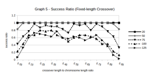Figure 6: Success Rates for different values of r (Fixed length Crossover function)

From Figure 6, it is evident that for cases where the Crossover length was less than 20% of the Chromosome length, the success rate was pretty bad. Same was the case when the Crossover length was more than 80% of the Chromosome length.

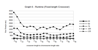Figure 7: Run Times for different values of r (Fixed length Crossover function)

In Figure 7, we see that very small crossover lengths (< 20% of the chromosome length) have a very large runtime compared to other crossover lengths.

4.1.2        Different Mutations

Success Rate: Figure 8 shows that FlipGA dominates the success chart with around 85% of success for instances with 125 variables. The alternative Multi bit greedy too is in par with FlipGA for most of the instances except the last set of instances, where its success rate drops to 75%. But keeping these two mutation functions aside, the rest of the mutation functions perform very poorly.

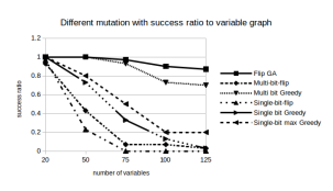Figure 8: Success Rates for different Mutation functions

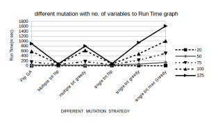Figure 9: Run Times for different Mutation functions

Runtime: Figure 9 shows that the runtime for Multi bit greedy is slightly better then FlipGA. So its like a trade off of accuracy over runtime. Perhaps increasing the MAX GEN value could improve the success ratio of Multi bit greedy without compromising the runtime to a great extent. Also, it might happen that for very large SAT instances the runtime difference betweeen these two functions might prove to be significant. The runtime of the rest mutation functions do not matter provided they have such a poor success rate.

Conflict of Interest The authors declare no conflict of interest.

Acknowledgment                 The authors would like to thank

Dr. Pinaki Mitra, Associate Professor, Department of CSE, IIT Guwahati for his invaluable contributions and support. We also thank him for the financial support he provided for the publication of this paper.

1. Peter Maandag. Solving 3-SAT (2012) http://www.cs.ru.nl/bachelorscripties/2012/PeterMaandag 3047121 Solving 3-Sat.pdf
2. Bart Selman, Hector Levesque, David Mitchell .A New Method for Solving Hard Satisfiability Problems(1992) www.cs.cornell.edu/selman/papers/pdf/92.aaai.gsat.pdf
3. Istvan Borgulya. An Evolutionary framework for 3-SAT Problem (2003) hrcak.srce.hr/file/69372
4. Stefan Harmeling. Solving Satisfiability Problems Using Genetic Algorithms (2000) https://pdfs.semanticscholar.org/70c0/6d4daabd3 75e818fb23cc6856fe271040095.pdf
5. Jens Gottlieb, Elena Marchiori, Claudio Rossi. Evolutionary Algorithms for the Satisfiability Problem (2002) www.cs.ru.nl/˜elenam/fsat.pdf
6. SATLIB-Benchmark Problems http://www.cs.ubc.ca/˜hoos/SATLIB/benchm.html
7. Random instance tough SAT Generator https://toughsat.appspot.com/
8. Elena Marchiori, Claudio Rossi. A Flipping Genetic Algorithm for Hard 3-SAT Problems (1999) https://pdfs.semanticscholar.org/e982/e6f15434d f6ecfd0b59cb45b7c6875744962.pdf

(Click to view)

(Click to view)