1.       Introduction

Most biological processes follow circadian rhythms, with the standard period of about 24 hours. These 24-hour rhythms are driven by circadian clocks, which have been observed in plants, fungi, cyanobacteria, and humans [1, 2]. In mammals, each cell contains molecular clocks, whose coordination is ensured by the suprachiasmatic nuclei in the hypothalamus through the generation of rhythmic physiology. Such a Circadian Timing System (CTS) regulates rhythmically cellular metabolism and proliferation over the 24 hours.

The body temperature follows circadian rhythms, that are tightly related to cancer development[3] [4]. Indeed, they play an important role in the coordination of molecular circadian clocks in various peripheral organs, such as lung, liver, kidney, and intestine, and could have an effect on tumors through their regulatory effects on Heat Shock Factor (HSF), Heat Shock Proteins (HSPs), and Cold-Induced Proteins [4, 5]. Moreover, it has been demonstrated that giving chemotherapy at an accurate circadian timing improves tolerance up to fivefold and to almost doubles antitumor efficacy, compared to constant rates or wrongly timed administrations, in both rodent models and cancer patients[6] [7]. In the same way, the destruction of the suprachiasmatic nuclei suppressed any circadian rhythm in body temperature in mice, which causes a 2-3 fold acceleration of experimental cancer progression [8]. On the other hand, the temperature circadian rhythms could be disrupted by anticancer medications, and molecular clocks are impaired, as a function of dose and circadian timing in mice [9, 10]. Therefore, the circadian rhythm of body temperature is a useful biomarker of CTS function[11] [12].

The relevance of monitoring core body temperature for CTS assessment has been approved in previous works, however they all suffer from a lack of non-invasive screening tools, which has limited testing in cancer patients [13, 14]. To overcome such a problem, one could use the skin temperature, which is correlated to core temperature. However, changes in skin temperature display an opposite pattern compared to that in core body temperature, but with a similar circadian rhythm.

In our work, a non-invasive wearable sensor, Movisens® GmbH, Karlsruhe, Germany, has been used. This sensor monitors skin temperature for up to 200 hours, with the sensor able to be worn at different positions such as the hip, wrist, or chest. The temperature signals are collected at a relatively low sampling frequency with this sensor, that is, one point every five minutes. Using such a low frequency is possible since temperature varies slowly over time. Also, a minimal memory is required and the battery life is extended, due to reduced energy consumption for the measurement device. However, having a low signal frequency produces more difficult complications. Moreover, sensor malfunction or a subject not wearing it for a period of time causes missing data in the signals.

This paper proposes an original algorithm to analyze the circadian rhythms in skin temperature signals. It first develops an interpolation algorithm to set the signals to a higher frequency such as one sample per minute, and to fill any gap in the signals [15]. For this reason, a kernel-based machine learning algorithm is presented and compared to other classic interpolation methods. Afterwards, a rhythmometric modeling, using Cosinor models, is proposed. It aims to extract parameters such as the MESOR, the amplitude, the orthophase and the bathyphase from interpolated signals. The paper then proposes a divergence study over these features to detect changes caused by chemotherapy. Five healthy subjects’ temperature signals are involved in this study, as a prerequisite for subsequent investigations involving a larger number in healthy controls and cancer patients.

2.       Subjects and Methods

2.1.  Subjects and materiel

In this study, three female and two male control subjects, aged 45.2 ±13.6 years, are considered. They were given a detailed description of the objectives and requirements of the study before the experiment, and they read and signed an informed consent prior to testing.  The infrared Movisens (GmbH – move III) sensor was positioned on the thorax of the subjects to monitor their skin temperature for four days. It measures 5.0 x 3.6 x1.7 cm³, and weighs 32 g. The sensor is composed of a tri-axial acceleration sensor (adxl345, Analog Devices; range: ±8 g; sampling rate: 64 Hz; resolution: 12 bit) embedded with a temperature sensor (MLX90615 high resolution 16bit ADC; resolution of 0.02°C). The recorded data is saved on a memory chip inside the sensor and transmitted to a server via GPRS. A hypoallergenic patch has been used to maintain the sensor in the upper right anterior thoracic area of the subjects.

2.2.   Interpolation of temperature signals

The temperature signals have a small frequency, with occasional missing data. Let  denote the temperature samples collected for a certain subject using the sensor, with  in minutes. The aim of interpolation is to estimate a function , that computes the temperature at any time , and which verifies the following:

Different algorithms for interpolation such as linear, polynomial or cubic splines techniques exist in the literature [15, 16]. In the linear interpolation, temperature is represented by a straight line between any two consecutive collected measurements. Having , for ,

This technique is easy to implement, but it yields several functions, one per interval between two consecutive measurements. Moreover, it is disadvantageous for large time-intervals due to the non-specification of the linear estimation. In the polynomial interpolation, temperature is represented by a single polynomial function, which fits the measured data. By using Lagrange polynomials, one obtains the following function:

where  is the degree of the obtained polynomial and . By taking  close to , the obtained function is specific, but with highly complex computations. Cubic splines is the most commonly used interpolation technique. It computes a set of piece-wise polynomial functions that maximize the smoothness of the whole curve. The -th splines function defined over the interval , for , is given as follows:

where  is the derivative of the temperature model . The values of the coefficients are then computed iteratively as shown in [2]. This technique is efficient, but proposes piece-wise functions, that need iterative computations.

•        Typical Reproducing Kernels

Kernel type	General expression
Gaussian
Polynomial
Exponential

This paper proposes a kernel-based regression approach that generates a single function [17, 18]. A training database is first constructed using the  collected temperature measurements . Then a model is computed using this database, taking time as input and yielding temperature as output. This model is defined using the kernel-based ridge regression technique. The model is afterwards applied to other times, where temperature values are unknown, for interpolation. Consider a reproducing kernel defined from to  and denote  its reproducing kernel Hilbert space. Some commonly used reproducing kernels are given in Table I. where the kernel parameters  and  are positive and  is a positive integer. Then the temperature model is defined by minimizing the regularized mean quadratic error between the model’s outputs and the measured data of the learning database:

where  is a regularization parameter that controls the tradeoff between the training error and the complexity of the solution and  is the norm in the reproducing kernel Hilbert space[19]. According to the Representer theorem, that all machine learning algorithms share, the minimization problem could be reduced to a more computation-friendly problem. Hence, the temperature model could be written as follows:

where the coefficients  are to be determined. Let  denote the column coefficients vector whose -th entry is . By injecting the model expression in the minimization problem, one obtains a dual optimization problem whose solution is given by:

where  is a -by-  matrix whose -th entry is given by ,  is the -by-  identity matrix and  is the temperature column vector, whose -th entry is given by . Now that the model  is defined for each temperature signal, the temperature value at a given time  is estimated by

The main advantage of the kernel-based approach remains in the fact that a single-function model is obtained, unlike the linear and cubic spline interpolations, where a piece-wise expression is obtained. In the following, and for simplicity, the notation  is used for the estimated signal, having a value at each minute, obtained after interpolation.

2.3.  Detection of rhythmicity

The detection of rhythmicity is usually performed in the frequency domain [20]. The spectral analysis using the “Fourier transform” is a well-known study to do this [21]. In this analysis, any signal, regardless of its shape and properties, can be represented by a complex function of frequency that highlights the frequencies that make it up. By applying the inverse Fourier transform, the signal is then decomposed into an infinite sum of sine and cosine functions of infinite frequencies [22]. The signals could be deterministic such as periodic/non-periodic or random such as stationary/non-stationary. A similar analysis for periodic signals is the Fourier series analysis, which represents a function as a sum of sine and cosine functions of different frequencies.

In this paper, an algorithm based on Fourier analysis is first proposed for frequency and harmonic detection. This algorithm starts by estimating the fundamental frequency, the fundamental amplitude and phase, and the harmonic amplitudes and phases, to evaluate the periodogram. The term periodogram was introduced by Schuster in December 1934 when Fourier analysis was used to estimate periodicity in meteorological phenomena [23]. The technique was evaluated for the first time when inspecting circadian rhythms in the 1950s to measure circadian rhythms of mice after blinding [24]. The periodogram showed that periodic signals have a frequency spectrum consisting of harmonics. For instance, if the time domain repeats at f, the frequency spectrum will contain a first harmonic at f, a second harmonic at 2f, a third harmonic at 3f, and so forth. The first harmonic, which is the frequency at which the time domain repeats itself, is called the fundamental frequency, and has the highest amplitude. Periodograms and spectral density were originally used in chronobiology in the 1960s [25].

In order to set the periodogram, a suitable window must be applied to the signal, to reduce side-lobes. For the proposed algorithm, a normalized Hanning window has been chosen [26] since this window does not disturb the position of spectral peaks in the spectral density, although the amplitude is decreased and the peak is larger. Having the periodogram and thus the fundamental and harmonic frequencies, the temperature signal is then modeled, using the Fourier series as follows:

where  is the angular frequency i.e. , i.e. is the fundamental period (duration of one cycle) and  is the number of the considered harmonics with the fundamental frequency. With respect to circadian rhythms, the rhythm persists in constant conditions with a period of around 24-hours, i.e.  minutes.  takes values from  to infinity. The higher  is, the better the model  fits the observed value . The parameters ,  and  could be computed using the computations of Fourier series. The main advantage of this technique is that one is able to determine the exact fundamental frequency, with its following ones, by analyzing the periodogram, obtained with the Fourier transform. However, it needs the data to be equidistant and to cover more than a single cycle, otherwise the analysis would be erroneous.

One interesting method used for analyzing unequidistant and time-limited observations is the single Cosinor procedure. This study was developed to evaluate rhythmicity of un-equidistant data series[27] [28], and is frequently used in the analysis of biologic time series that have expected rhythms. Cosinor uses the least squares method to fit a sum of sine functions to a time series, as least squares procedures do not have an equidistant data limitation. Practically, it considers the Fourier series model of (8) with a precise fundamental frequency, which corresponds to 24-hours, and number of harmonics and then computes the parameters ,  and  so as to minimize the error between the signal  and the model . Let be the residual corresponding to the value , that is,

and consider the modeling error as the sum of the squared residuals ( ) for all the data, that is,

The parameters ,  and  are then obtained using least squares by setting the derivatives of the  over each parameter equal to zero. Since the temperature follows a circardian rhythm, then the fundamental frequency corresponds to 24h. Figure 1 shows an example of a Cosinor model obtained with . The obtained model will subsequently be used to compute significant rhythmometric parameters, as shown in the following paragraph.

Once the temperature signals are modeled, using either Fourier series or Cosinor, some features are extracted from their sinusoidal representation, as will be shown in the following paragraph.

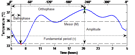Figure 1 Circadian Rhythm Model

2.4.  Features selection and divergence study

Once the temperature signal is decomposed into cumulative sine functions, using Fourier series or Cosinor, the objective here is to determine the sinusoidality of the data. This requires the extraction of some features from the models by inspecting their graph plotted against time, as shown in Figure 1. When the model is composed of more than one trigonometric function, that is, the fundamental period and some harmonics, four features could be extracted [29]:

• the MESOR (M), for “Midline Estimating Statistic Of Rhythm”, that is the mean of the model,

• the amplitude (A) that is defined as the half of the difference between the maximum and the minimum of the model in one fundamental period,

• and, finally, the phases of the maximum and the minimum of the composite model including harmonic terms, which are called the orthophase Φ_O and bathyphase Φ_B

Figure 1 illustrates these features. For a control subject, these rhythmometric parameters vary slightly over time; whereas chemotherapy could produce significant modification in the circadian rhythm, which yields a divergence of one or more rhythmometric parameters. In order to detect this divergence, a sliding window algorithm is considered over the temperature signal  of a period of several days.

Then, for each window, the signal is modeled using the cumulative sine functions, and the four rhythmometric parameters are extracted. A statistical test, such as an exact Fisher test, Wilcoxon test or another, is then applied to check whether the values through the window diverge from their previous values. This study is motivated by the perturbation of the circadian rhythm due to chemotherapy, which induce a divergence of the statistical distributions of the extracted rhythmometric parameters.

3.       Results

This section starts with the illustration of the effectiveness of the interpolation techniques. To this end, the collected temperature signals of two subjects out of the five are considered. These two have a frequency of one sample per minute over four days, whereas the remaining are measured with a rate of one sample every five minutes. An example of a skin temperature signal while wearing the IR sensor for four days, for a control pattern with an expected pattern is shown in Figure 2.

Table II. Interpolation results

Interpolation methods	Interpolation mean error ± SD
	0 segment removed	1 segment removed	2 segments removed	3 segments removed
Linear	0.13±0.7	0.16±0.8	0.18±0.7	0.19±0.8
Cubic splines	0.15±0.7	0.17±0.8	0.19±0.8	0.25±0.9
Polynomial	0.80±1.4	0.80±1.4	0.81±1.4	0.81±1.4
Kernel-based	0.06±0.2	0.08±0.3	0.11±0.3	0.13±0.4

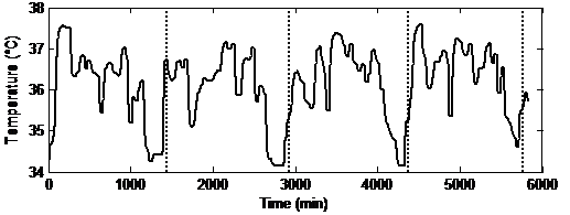Figure 2 Skin temperature signal

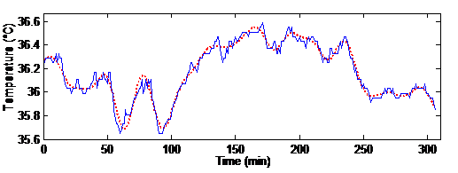Figure 3 Kernel-based interpolation signal (dashed line) and its true measured one (straight line) for one subject over five hours, i.e. 300 minutes

In order to compare the interpolation approaches, the signals of the two subjects were divided into segments of 1440 minutes, i.e. one-day length, leading to eight segments. Then, these segments are resampled by taking one point every five minutes, leading to segments of 288 points. Thereafter, the linear, polynomial, cubic spline and kernel-based interpolation techniques were applied over these segments and the results are compared to the original observed signal. For the kernel-based interpolation, a Gaussian kernel was used, using a cross-validation algorithm to select the optimal values of the bandwidth  and the regularization parameter  according to the learning data [17]. The mean errors for the interpolations are shown in Table II. These were computed by averaging the absolute difference between the observed and the estimated signals for the eight segments. In order to simulate the missing data, a 30-min segment was subsequently removed from the one-day length segment. This 30-min segment corresponds to six consecutive points among the 288-point segments. Then, two and three 30-min segments are removed. These segments were randomly selected within each one-day length segment. Table II shows the results for segments with no missing data (0 segment removed), one 30-min segment removed, two segments removed, and three segments removed. It is worth noting that simulations are performed 50 times and errors are averaged over all results, since the removed segments are selected randomly. The table shows that the Kernel-based algorithm yields better results with less estimation error in all cases, which is expected due its malleability and its adaptation to the curve, even under non-linear conditions.

The measured temperature signal for a typical subject for a five-hour period is shown in Figure 3. The figure also shows the interpolated signal obtained with the kernel-based interpolation.

Table III. Rhythmometric parameters Mean (±SD) Fourier series (24h) Fourier transform ( ) Cosinor model (24h) Orthophase 96.9±0.6 104.1±1 97.8±0.5 Bathyphase 27.58±0.8 38.8±0.8 28.4±0.5

The plot shows that the computed signal is close to the measured one, with a smooth curve produced.

Then, the objective is to illustrate the rhythmometric modeling techniques, which use the Fourier series or Cosinor. To this end, we consider the 5 temperature signals over a 4-day period, having passed the interpolation phase, i.e. the signals have no gaps, with a rate of one sample per minute. We start by applying the Fourier series, taking the fundamental period to be equal to 24 hours, i.e. 1440 minutes, followed by 3 harmonics, i.e. 12 hours, 8 hours and 6 hours. We consider that the modeling error is the average of the absolute differences between the 4-day temperature signals and their modeled ones for the 5 signals. In this case, the modeling error of the Fourier series technique with a 24-hour period is equal to 0.77. We then apply the Fourier transform to the signals to obtain their periodograms. These computations showed that the local maxima of the spectral energy are not obtained exactly at the frequencies 1/24, 1/12, 1/8 and 1/6, but very close to them.

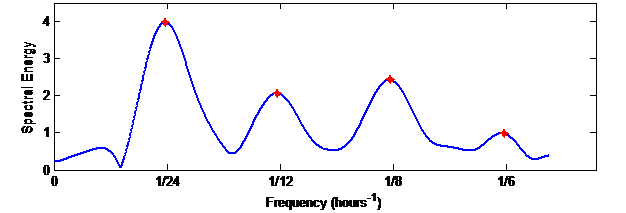Figure 4 Periodogram generated by the Fourier analysis of the time series

Figure 4 shows a periodogram obtained for a certain subject, where the fundamental frequency is equal to 1/23.5. Let be the fundamental period obtained by taking the maximal point of the periodogram, i.e.  is very close to 24 hours. If we take  and the following three local maxima, and perform the inverse Fourier transform, the modeling error decreases to 0.73, which was expected since this way more information is considered in the modeling. Having the fundamental period not equal to 24h is related to the fact that only four cycles (4 days) are considered, which is not enough for Fourier analysis. Afterwards, by applying Cosinor computations, while taking the fundamental period equal to 24h, and considering the following 3 harmonics, the modeling error is the least, being equal to 0.53. This shows the power of such a method with limited-duration signals.

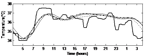Figure 5 Temperature modeled signals using the Fourier series with a 24h period in thin dashed line, the Fourier transform with a 23.5h period in thin straight line and the Cosinor in thick dashed line, and the original signal in thick straight line.

Figure 5 shows the modeled signals in a thin dashed line for the Fourier series using a 24h period, a thin straight line for the Fourier transform using a 23.5h period and a thick dashed line for the Cosinor analysis. It also shows the original signal in thick straight line, for a one day period going from 5 a.m. till 5 am. the following day. The curves show that the obtained signals follow the original one with a small modeling error. The rhythmometric parameters, i.e. orthophase and bathyphase, are then computed. Table III shows their mean values in degrees with the standard deviations over the 5 signals. Here the parameters are extracted from the rhythmometric models obtained for the whole 4-days signals. As expected, considering the fundamental period  from the periodogram, modeling leads to a difference in the characteristics equivalent to 30 minutes, whereas both Fourier series and Cosinor lead to close values. This study shows that the Cosinor computations have promising results, to be validated with more signals later on.

4.       Discussion

This paper proposed a longitudinal evaluation of skin temperature measurement, collected using a thoracic sensor. The collected signals have a sampling frequency of one point every five minutes, with a length of four days for control subjects. At a first phase, we performed interpolation, using a kernel-based machine learning technique, to resample the signals to a higher frequency of one point every minute and to fill in the gaps in the measured signals. This step is crucial for the following data processing techniques. A rhythmometric study is then followed up on resampled signals, using either a Fourier representation or Cosinor. A Fourier analysis with the Fourier transform and the Fourier series is first proposed to model the signals, then a Cosinor model is constructed using Fourier analysis and least squares computations. The advantage of Cosinor remains in its robustness against un-equidistant and low-duration data, which is not the case for Fourier analysis. Rhythmometric parameters such as MESOR, amplitude, orthophase and bathyphase, are then extracted using the obtained model. For a given temperature signal of a given subject, such computations are performed for each sliding window of the signal, leading to a set of random variables that are the rhythmometric parameters. Then a divergence study is applied to detect any perturbation of the rhythm. In fact, chemotherapy can alter the circadian rhythm of the patients, therefore it is expected in that case to observe a divergence of the distributions of the rhythmometric parameters between the time span on chemotherapy and that before or after it. To detect such divergence, we can separate each parameter values into two sets (on or off chemotherapy), then apply a statistical test to detect the divergence between their distributions. This study is promising since chemotherapy-induced perturbations have been documented for over 15 anticancer drugs in experimental models, and for several drug combination protocols in cancer patients [6 14 15].

The kernel-based interpolation phase was validated using different cases of missing data in the signals, and by comparing them to well-known interpolation methods such as linear, polynomial and cubic splines. A comparison between the rhythmometric modeling techniques is then conducted, showing that Cosinor analysis leads to fewer modeling errors. Having only five signals with a 4-day duration is not enough to draw conclusions, however the results are promising for future works. Thus a larger study involving more healthy controls and cancer patients is planned to further determine the relevance of the methodology developed here and the minimum number of harmonics. It should be possible to evaluate the effect of harmonics such as 12h, 8h, and 6h, and even to use only specific harmonics of varying frequency in order to determine the exact moment when the circadian rhythm is modified. Advanced processing such as the goodness of fit and the rhythm detection will also be applied on the signals using the F-test. Moreover, an evaluation of the IR sensor is also to be done, to verify if the observed temperature with such a sensor remains a mirror of the central temperature.

5.       Acknowledgments

The authors would like to thank all clinicians, clinical research associates and technicians for their involvement in the device design and the protocol definition, set-up and monitoring. This work was supported by the Champagne-Ardenne Regional Council; PICADO project (Projet Innovant pour le Changement d’Ampleur de la Domomédecine).

1. Panda, S., Hogenesch, J.B., and Kay, S.A.: ‘Circadian rhythms from flies to human’, Nature, 2002, 417, (6886), pp. 329-335
2. Edgar, R.S., Green, E.W., Zhao, Y., van Ooijen, G., Olmedo, M., Qin, X., Xu, Y., Pan, M., Valekunja, U.K., Feeney, K.A., Maywood, E.S., Hastings, M.H., Baliga, N.S., Merrow, M., Millar, A.J., Johnson, C.H., Kyriacou, C.P., O/’Neill, J.S., and Reddy, A.B.: ‘Peroxiredoxins are conserved markers of circadian rhythms’, Nature, 2012, 485, (7399), pp. 459-464
3. Greene, M.W.: ‘Circadian rhythms and tumor growth’, Cancer Letters, 2012, 318, (2), pp. 115-123
4. Li, X.-M., Delaunay, F., Dulong, S., Claustrat, B., Zampera, S., Fujii, Y., Teboul, M., Beau, J., and Lévi, F.: ‘Cancer Inhibition through Circadian Reprogramming of Tumor Transcriptome with Meal Timing’, Cancer Research, 2010, 70, (8), pp. 3351-3360
5. Reinke, H., Saini, C., Fleury-Olela, F.., Benjamin, I.J., and Schibler, U.: ‘Differential display of DNA-binding proteins reveals heat-shock factor 1 as a circadian transcription factor’, Genes Dev, 2008, 22, (3), pp. 331-345
6. Levi, F., Altinok, A., Clairambault, J., and Goldbeter, A.: ‘Implications of circadian clocks for the rhythmic delivery of cancer therapeutics’, Philos Trans A Math Phys Eng Sci, 2008, 366, (1880), pp. 3575-3598
7. Levi, F., Okyar, A., Dulong, S., P.F., and Clairambault, J.: ‘Circadian timing in cancer treatments’, Annu Rev Pharmacol Toxicol, 2010, 50, pp. 377-421
8. Filipski, E., Li, X.M., and Levi, F.: ‘Disruption of circadian coordination and malignant growth’, Cancer Causes Control, 2006, 17, (4), pp. 509-514
9. Ahowesso, C., Li, X.M., Zampera, S., Peteri-Brunback, B., Dulong, S., Beau, J., Hossard, V., Filipski, E., Delaunay, F., Claustrat, B., and Levi, F.: ‘Sex and dosing-time dependencies in irinotecan-induced circadian disruption’, Chronobiol Int, 2011, 28, (5), pp. 458-470
10. Ohdo, S., Koyanagi, S., Suyama, H., Higuchi, S., and Aramaki, H.: ‘Changing the dosing schedule minimizes the disruptive effects of interferon on clock function’, Nat Med, 2001, 7, (3), pp. 356-360
11. Innominato, P.F., Roche, V.P., Palesh, O.G., Ulusakarya, A., Spiegel, D., and Lévi, F.A.: ‘The circadian timing system in clinical oncology’, Annals of Medicine, 2014, 46, (4), pp. 191-207
12. Scully, C.G., Karaboué, A., Liu, W.-M., Meyer, J., Innominato, P.F., Chon, K.H., Gorbach, A.M., and Lévi, F.: ‘Skin surface temperature rhythms as potential circadian biomarkers for personalized chronotherapeutics in cancer patients’, Interface Focus, 2011, 1, (1), pp. 48-60
13. Ortiz-Tudela, E., Martinez-Nicolas, A., Campos, M., Rol, M.A., and Madrid, J.A.: ‘A new integrated variable based on thermometry, actimetry and body position (TAP) to evaluate circadian system status in humans’, PLoS Comput Biol, 2010, 6, (11), pp. e1000996
14. Duffy, J.F., Dijk, D.-J., Klerman, E.B., and Czeisler, C.A.: ‘Later endogenous circadian temperature nadir relative to an earlier wake time in older people’, American Journal of Physiology – Regulatory, Integrative and Comparative Physiology, 1998, 275, (5), pp. R1478-R1487
15. Flores-Tapia, D., Thomas, G., and Pistorius, S.: ‘A comparison of interpolation methods for breast microwave radar imaging’, Conf Proc IEEE Eng Med Biol Soc, 2009, 2009, pp. 2735-2738
16. Chang, N.F., Chiang, C.Y., Chen, T.C., and Chen, L.G.: ‘Cubic spline interpolation with overlapped window and data reuse for on-line Hilbert Huang transform biomedical microprocessor’, Conf Proc IEEE Eng Med Biol Soc, 2011, 2011, pp. 7091-7094
17. Mahfouz, S., Mourad-Chehade, F., Honeine, P., Farah, J., and Snoussi, H.: ‘Kernel-based machine learning using radio-fingerprints for localization in wsns’, Aerospace and Electronic Systems, IEEE 2015, 51, (2), pp. 1324-1336
18. Vapnik, V.N.: ‘The nature of statistical learning theory’ (Springer-Verlag New York, Inc., 1995. 1995)
19. Aronszajn, N.: ‘Theory of reproducing kernels’, Trans. Amer. Math. So, 1950, 68 pp. 337-404
20. Michel Cosnard, J.D., Alain Le Breton ‘Rhythms in Biology and Other Fields of Application : Deterministic and Stochastic Approache’ (1983. 1983)
21. Bloomfield, P.: ‘Fourier Analysis of Time Series: An Introduction, ’ (New York ;Wiley 2000, . )
22. Fourier, J.B.J.: ‘Théorie analytique de la chaleur’ (1822. 1822)
23. Bartels, J.: ‘Arthur Schuster’s work on periodicities’, Terrestrial Magnetism and Atmospheric Electricity, 1934, 39, (4), pp. 345
24. Halberg, F., Visscher, M.B., and Bittner, J.J.: ‘Relation of visual factors to eosinophil rhythm in mice’, Am J Physiol, 1954, 179, (2), pp. 229-235
25. Panofsky, H., & Halberg, F.: ‘Thermo-variance spectra; simplified computational example and other methodology. II’, Exp Med Surg, 1961, 19, pp. 323-338
26. Nuttall, A.: ‘Some windows with very good sidelobe behavior’, IEEE Transactions on Acoustics, Speech, and S. Processing, 1981, 29, (1), pp. 84-91
27. Cornelissen, G.: ‘Cosinor-based rhythmometry’, Theoretical Biology & Medical Modelling, 2014, 11, pp. 16-16
28. Halberg, F., Tong, Y.L., and Johnson, E.A.: ‘Circadian System Phase – an aspect of temporal morphology : procedures and illustrative examples’ (Springer-Verlag, 1965. 1965)
29. Bingham, C., Arbogast, B., Guillaume, G.C., Lee, J.K., and Halberg, F.: ‘Inferential statistical methods for estimating and comparing cosinor parameters’, Chronobiologia, 1982, 9, (4), pp. 397-439

(Click to view)

(Click to view)

No. of Downloads Per Month

No. of Downloads Per Country