Spatiotemporal Traffic State Prediction Based on Discriminatively Pre-trained Deep Neural Networks
Spatiotemporal Traffic State Prediction Based on Discriminatively Pre-trained Deep Neural Networks
Volume 2, Issue 3, Page No 678-686, 2017
Author’s Name: Mohammed Elhenawy1, Hesham Rakha2, a)
View Affiliations
1Postdoctoral associate with the Center for Sustainable Mobility, Virginia Tech Transportation Institute, VA, 24061, USA
2Director of the Center for Sustainable Mobility (CSM) at the Virginia Tech Transportation Institute (VTTI), USA
a)Author to whom correspondence should be addressed. E-mail: hrakha@vt.edu
Adv. Sci. Technol. Eng. Syst. J. 2(3), 678-686 (2017); ![]() DOI: 10.25046/aj020387
DOI: 10.25046/aj020387
Keywords: Traffic state prediction, Proactive decision support systems, Deep Neural Network

Export Citations
The availability of traffic data and computational advances now make it possible to build data-driven models that capture the evolution of the state of traffic along modeled stretches of road. These models are used for short-time prediction so that transportation facilities can be operated in an efficient way that guarantees a high level of service. In this paper, we adopted a state-of-the-art machine learning deep neural network and the divide-and-conquer approach to model large road stretches. The proposed approach is expected to be a tool used in daily routines to enhance proactive decision support systems. The proposed approach maintains spatiotemporal correlations between contiguous road segments and is suitable for practical applications because it divides the large prediction problem into a set of smaller overlapping problems. These smaller problems can be solved in a reasonable time using a medium configuration PC. The proposed approach was used to model 21.1- and 30.7-mile stretches of highway along I-15 and I-66, respectively. The resulting predictions were better than predictions obtained using partial least squares regression.
Received: 13 April 2017, Accepted: 12 May 2017, Published Online: 05 June 2017
1. Introduction
The growing economy and an increasing number of vehicles on the road have brought about traffic problems that increase travelers’ inconvenience. Traffic congestion features prominently among these problems, and has become an everyday concern in many urban areas, bringing with it negative environmental effects. During periods of congestion, cars cannot run efficiently, resulting in air pollution, carbon dioxide (CO2) emissions, and increased fuel use. In 2007, wasted fuel and lost productivity cost Americans $87.2 billion. This number reached $115 billion in 2009 [1]. Congestion also increases travel time. In 1993, driving under congested conditions caused a delay of about 1.2 minutes per kilometer of travel on arterial roads [2]. Since then, this problem has grown worse, as evidenced by a report from the Texas Transportation Institute that indicates that the number of wasted hours due to traffic congestion increased fivefold between 1982 and 2005 for Americans.
In the past, the solution to these problems was constructing new roads, but that era of build-out ended due to its social and economic effects. Subsequently, Transportation Management Centers (TMCs) were deployed to solve traffic problems. Most of these TMCs operate in reactive mode, applying management strategies only after conditions in their regions change. Today, due to advances in technology, applying predictive traffic control strategies offers a cost-effective solution to improving traffic flow. Predictive traffic control is a proactive approach where traffic problems, such as congestion, are anticipated and countermeasures are applied prior to their occurrence.
Data-driven, short-term prediction of traffic characteristics, such as flow, density, and speed, is essential for applying predictive traffic control strategies. However, because of unstable traffic conditions and complex road settings, short-term prediction is not a straightforward task [3]. Applying mathematical models that are based on macroscopic and microscopic theories of traffic flow is difficult so data-driven modeling is considered a good approach to model complex traffic characteristics. Thanks to computational advances that make data collection and processing easy and rapid, a promising research area based on data-driven algorithms has emerged.
The use of deep learning neural networks for traffic state prediction was demonstrated to be promising by Elhenawy and Rakha [4]. In this paper, we describe new research on the prediction of traffic speeds and flows for basic freeway segments using a data-driven approach. Predictions are based on the current traffic state data, weather conditions, visibility levels, and seasonal predictors (i.e., day of the week and time of the day). State-of-the-art deep neural networks were trained and tested to predict traffic states for a larger spatial and temporal horizon. The proposed approach allows for identification of traffic problems up to 2 hours in advance, and implementation of solutions up to several miles away. In order to make the proposed approach suitable for practical applications at TMCs, a principal component analysis (PCA) was used to reduce the dimensionality of the inputs to the deep neural network. Moreover, we used the divide-and-conquer approach to divide the large prediction problem into a set of smaller overlapping problems.
Following the introduction, in Section 2 related work is discussed. Section 3 defines the short-term prediction problem. Section 4 briefly presents a background of the methods used in this paper. The model calibration is described in Section 5. The study sites and the preprocessing of the traffic state data are discussed in Section 6. In Section 7, the results of the experimental work are outlined. Finally, the paper’s conclusions and recommendations for future work are described in Section 8.
2. Related Work
Over the past few decades, traffic characteristic prediction models have been developed by researchers from different areas, such as transportation engineering, control engineering, and economics. The developed prediction approaches can be classified into three broad categories: parametric models, nonparametric models, and simulations. Parametric models include time-series models, stochastic differential equations, etc. Nonparametric models include a variety of techniques that range from simple methods like k-nearest neighbor (k-NN) to complex support vector regressions (SVR) and artificial neural networks (ANNs).
The time-series technique is a parametric model used widely in traffic flow prediction. The autoregressive integrated moving average (ARIMA) model was used very early to predict short-term freeway traffic flow [5]. After that, different advanced versions of ARIMA were used to develop more-accurate prediction models. Voort et al. integrated the Kohonen self-organizing map and ARIMA into a new method called KARIMA, which uses a Kohonen self-organizing map to cluster the data and then models each cluster using ARIMA [6]. Lee et al. used a subset ARIMA model for the one-step-ahead forecasting task, which returned more stable and accurate results than the full ARIMA model [7]. Williams and Hoel used seasonal ARIMA (SARIMA) to analyze data from two freeways, and the results showed that one-step seasonal ARIMA predictions outperformed heuristic forecast benchmarks [8].
Due to both the highly nonlinear nature of traffic characteristics and the availability of data, nonparametric methods have also attracted researchers’ attention. For traffic flow prediction, there are many versions of the k-NN algorithm that show a good prediction accuracy. Davis and Nihan argued that k-NN can capture linear and nonlinear relationships and is therefore able to model the nonlinear transition between free-flow and congested traffic [9]. However, the results of their empirical study showed that k-NN was no better than a simple univariate time-series forecast. Sun et al. considered the traffic prediction model as a nonlinear system with historical and current traffic characteristics as inputs and future traffic characteristics as outputs [10]. They used the local linear regression model to approximate the nonlinear relationship between system inputs and outputs to predict future traffic characteristics. Young-Seon et al. proposed a short-term traffic flow prediction algorithm combining the online-based SVR with the weighted learning method for short-term traffic flow predictions [1]. ANN is considered one of the best tools to model highly nonlinear relationships between inputs and outputs, and many papers have adopted different ANN models, such as the Bayesian neural network [11] and radial basis function neural network [12], for predicting traffic flow. For more information, Vlahogianni et al. [13] provide a good review of the proposed techniques as well as the challenges of short-term prediction.
Recently, a number of algorithms have been developed to train neural networks with many hidden layers. These deep learning neural networks are state-of-the-art machine learning techniques used to solve complex problems. However, this technique requires a huge amount of data for the training to return good results. In recent years, deep neural networks have attracted the attention of researchers in the transportation field as a super-tool to model traffic evolution. Huang et al. used a deep belief network to learn the important features for flow prediction and then passed those features to the regression output layer [14]. In another paper, the problem of traffic forecasting at peak hour and after an accident is approached using a generic deep learning framework based on long short term memory units [15]. Polson and Sokolov used a deep neural network to predict traffic flow, demonstrating that the deep neural network is capable of giving precise short-term prediction at the sharp traffic flow regime [16]. Lv et al. used a stacked autoencoder model to learn features that capture the nonlinear spatial and temporal correlations from the traffic data, then forwarded these features to the output layer to predict the traffic flow [17]. In an another recent study by Ma et al., spatiotemporal speed matrices were considered as images and used to train a convolution neural network, and then this network was used to predict large-scale, network-wide traffic speed with high accuracy [18].
3. Problem Definition
In this research, we are interested in predicting the traffic states of several segments of a freeway for up to a 2-hour horizon. This is not an easy task, since the evolution of traffic states is a complex spatiotemporal process. In order to define our prediction problem, we first define the spatiotemporal speed/flow matrix, , where I is the number of the stretch’s segments and T is the day’s time intervals. The spatiotemporal traffic state prediction problem can be stated as follows. Let be the observed elements of the spatiotemporal state matrix at the time interval and segment of the studied stretch of road. Given the spatiotemporal observed traffic state submatrix that ends at time , the forecasted weather conditions, and the visibility level, our goal is to predict the spatiotemporal traffic state submatrix that spans the time interval for some prediction horizon .
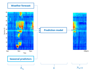
Figure 1. Illustration of the problem where a model is needed to predict the speed evolution in time (x-axis ) and space (y-axis ).
The general form of the solution for the problem above is shown in Equation 1 [19];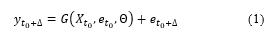
where:
| the chosen model | |
| the prediction at horizon | |
| the inputs’ predictors, including the observed elements of the spatiotemporal state submatrix at the time interval , time of day, day of week, and the forecasted weather conditions and visibility | |
| estimated model parameters | |
| errors (unexplained variability) due to the absence of factors we cannot observe |
We propose using a deep neural network for this prediction problem for the following three reasons. First, the stochastic nature of the input-output data makes it possible to find two different responses for the same input. In other words, the response corresponding to any input predictor is a distribution rather than a single point in the response space. Second, the spatiotemporal response is multivariate and the input-output relationship is nonlinear. Third, there is no closed mathematical form (model) that can be used to explain the relationship between the input predictors and the response.
4. Methods
4.1. Discriminatively Pre-Trained Deep Neural Networks
In machine learning, ANNs are powerful tools used to estimate or approximate unknown linear and nonlinear functions, and are used for both classification and regression problems.
An ANN consists of an input layer, hidden layers, and an output layer. Each layer consists of several processing units, called neurons. In this paper, we used a multi-layered, feed-forward ANN, which is commonly used for classification/regression analysis. In a multi-layered, feed-forward ANN, the neurons make use of directed connections, which allow information flow in the direction from the input layer to output layer. A neuron at layer receives an input from each neuron at layer . The neuron adds the weighted sum of its inputs to a bias term, then applies the whole thing to a transfer function and passes the result to its output toward the downstream layer. Given the training dataset, the ANN can use a learning algorithm such as back propagation to learn the weights and biases for each single neuron [20]. In general, training a deep neural network that has more than one hidden layer is challenging because the gradient vanishes as it propagates back. Over the past 10 years or so, many algorithms have been proposed to train deep neural networks, the discriminative pre-training method being one of the most simple [21]. The discriminative pre-training algorithm starts by training a neural network that has only one hidden layer. The input predictors and the responses are used in the supervised pre-training. Once the one-hidden-layer network has been trained, the algorithm inserts a new hidden layer before the output layer. The expanded whole network keeps the weights and biases of the input layer and the previously pre-trained hidden layer as initial weights for the next pre-training cycle. This algorithm continues growing the network until the desired depth is reached. Finally, the whole network is fine-tuned using a backpropagation algorithm.
4.2. Partial Least Squares Regression
Multiple linear regression (MLR) is a good tool to model the relationship between predictors and responses. MLR is effective when the number of predictors is small, there is no significant multicollinearity, and there is a well-understood relationship between predictors and responses [22]. In many scientific problems, the relationship between predictors and responses are poorly understood, and the main goal is to construct a good predictive model using a large number of predictors. In this case, MLR is not a suitable tool. If the number of predictors becomes too large, an MLR model will over-fit the sampled data perfectly but fail to predict new data well.
When the number of the observations is less than the number of predictors, the chance of multicollinearity increases and ordinary MLR fails. Several approaches have been proposed to overcome this problem. For instance, principal component regression is used to remove the multicollinearity by projecting X into the orthogonal component and then regressing X’s scores on Y. These orthogonal components explain X but may not be relevant for Y.
Partial least squares regression (PLSR) is a more recent technique that generalizes and combines features from principal component analysis and MLR. It is used to predict Y from X and to describe their common structure. PLSR assumes that there are a few latent factors that account for most of the variation in the response. The general idea of PLSR is to try to extract those latent factors, accounting for as much of the predictors’ X variation as possible, while at the same time modeling the responses well. A number of variants of PLSR algorithms exist, most of which estimate the coefficients of the linear regression between and as . Some PLSR algorithms are designed for the case where is a column vector, while others are suitable for the general case, in which is a matrix. One example of a simple PLSR algorithm is the nonlinear iterative partial least squares (NIPALS) algorithm [23].
4.3. Principal Component Analysis (PCA)
The stretch-wide prediction problem is a multivariate problem that may involve a considerable number of correlated predictors. PCA is a popular technique for dimensionality reduction that linearly transforms possibly correlated variables into uncorrelated variables called principal components.
PCA is usually used to reduce the number of predictors involved in the downstream analysis; however, the smaller set of transformed predictors still contains most of the information (variance) in the large set. The principal components are the Eigenvectors of the dataset covariance matrix. The following steps show how to find principle components given data vectors in the space where .
- Normalize input data vectors.
- Compute the covariance matrix for the normalized dataset.
- Compute the Eigenvectors and the associated Eigenvalue of the covariance matrix .
- Sort the Eigenvectors in order of decreasing Eigenvalues.
- Reduce the size of the data by choosing the first
- Construct a good approximation of the original dataset by multiplying the transpose of the matrix consisting of the Eigenvectors with the original data matrix.
The first principal component is the normalized Eigenvector, which is associated with the highest Eigenvalue. The first principal component represents the direction in the space that has the most variability in the data, and each succeeding component accounts for as much of the remaining variability as possible.
5. Model Calibration
5.1. Divide-and-Conquer Approach
One major challenge in traffic state short-term prediction using the spatiotemporal state matrix is the dimension of the predictor and response vectors and the large number of required parameters that must be estimated. As the stretch of road grows, the deep neural network needs a great deal of time for training or suffers from memory problems. To deal with these issues, this study adopts a divide-and-conquer approach model.
The divide-and-conquer paradigm suggests that if the problem cannot be solved as is, it should be decomposed into two or more small problems of the same type, which are then solved. The final solution to the difficult big problem is the combination of solutions to the smaller problems.
We applied divide and conquer in a straightforward manner to our prediction problem by dividing the input predictors of the spatial-temporal state matrix into smaller overlapping windows. The same method was applied to the responses, as shown in Figure 2.
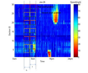
Figure 2. Illustration of divide-and-conquer approach, where l is the prediction horizon and h is the width of the predictors’ windows.
The overlap of the windows is important for determining a smooth predicted speed. In the experimental work done in this paper, we set the window length equal to four segments and the overlap between contiguous windows equal to two segments. Because of this overlap between windows, each segment has two predicted traffic states at the testing phase, and the final predicted traffic state for overlapped segments is the average.
1.1. Training and Testing Phase
The model calibration process consists of a training phase and a testing phase. In the training phase, the deep neural network’s weights are estimated using the training dataset. In the testing phase, the constructed deep neural network’s accuracy is tested using an unseen dataset called the testing dataset. The training phase in our approach includes the following steps:
- Partitioning (dividing) the whole stretch into small windows, each with four segments.
- Preparing the and matrices for each window by reshaping the traffic state, weather, and visibility inside the windows, with widths of and
- Shifting the window to the right and repeating Step 2 to get another raw and , as shown in Figure 3.
- Using PCA to find , which is the scores of the matrix .
- Using and matrices as the inputs and outputs, respectively, to train the one-hidden-layer neural network. Once the one-hidden layer network is trained, the algorithm discards the output layer and keeps the first hidden layer with its trained weights. Then, it stacks another hidden layer with a new output layer on top of the first layer and randomly initializes the weights of the new layers. The grown network is retrained again using the same and This algorithm continues growing the network until the desired depth is reached. Finally, the whole network is fine-tuned using the backpropagation algorithm.
Figure 3. Illustration of preparing X and Y matrices for one window.
The testing phase is always simpler and does not require a great deal of time. This phase includes passing the testing data through the neural network after reducing it using the same principal components. The last step in testing is putting the predicted pieces together to find the prediction for the whole stretch.
6. Case Study
The performance of the proposed algorithm was tested on two real datasets collected from Interstate 66 (I-66) in Virginia and Interstate 15 (I-55) in California. This section describes the study sites and the preparation of the data.
6.1. Virginia Study Site
The selected I-66 eastbound study site is located between Gainesville and Arlington in Northern Virginia. There are 36 segments along the selected 30.7-mile stretch of freeway. This corridor has four lanes in each direction, with the leftmost lane designated as an HOV-2 lane during morning and afternoon peak hours. This is the major commuting corridor between Northern Virginia and Washington, DC. INRIX probe data from 2011 to 2013 were used to develop the prediction models, and data reduction was conducted to extract the daily traffic speed matrices. One-minute average speeds (or travel times) are available in the raw data for each roadway segment. Initially, the daily speed data were sorted by time and location from the raw data into a two-dimensional matrix. In order to reduce the stochastic noise and measurement error, the speed matrices were aggregated by 15-minute intervals. The missing data in the aggregated speed matrices were estimated using the moving average from a 3 × 3 window.
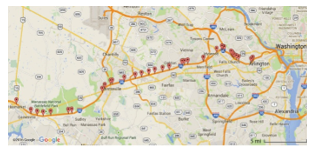
Figure 4. Virginia study site (I-66) (source: Google Maps).
6.2. California Study Site
The 2013 and 2014 loop detector data from I-15 southbound were used to develop traffic prediction models for the California study site. The layout of the I-15 freeway corridor and the locations of loop detectors are presented in Figure 4. There are 43 loop detectors along the 21.1-mile stretch of the corridor. Data reduction was conducted on the loop detector data collected from the test site to extract the daily traffic data matrices of speed and flow. The speed and flow matrices were 15-minute aggregated matrices.
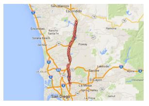
Figure 5. California study site (I-15) (source: Google Maps)
7. Prediction Experimental Results
This section describes the evaluation criteria and then shows the experimental results of the proposed traffic state prediction for the Virginia and California study sites.
7.1. Evaluation Criteria
Relative and absolute prediction errors were calculated to compare the models using shallow networks, those using deep neural networks, and those using PLSR. The relative error was computed as the Mean Absolute Percentage Error (MAPE) using (2). This error is the average absolute percentage change between the predicted and the true values. The corresponding absolute error is presented by the mean absolute error (MAE) using (3). This error is the absolute difference between the predicted and the true values.
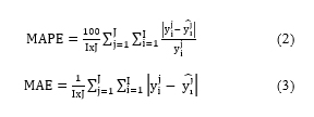
where:
J = total number of observations in the testing data set
I = total number of elements in each observation
y = ground truth traffic state
= predicted traffic state
In the following experimental work, leave-one-out validation was used to cross-validate the prediction errors. During each fold of the leave-one-out validation, one month was kept out for testing and the other months were used to train the model such that each month was used only once for testing. The leave-one-out validation subsequently reported the final prediction errors as the average errors of all folds.
7.2. I-66 Results
In this section, we present the results of applying the PLSR model, shallow network model, and deep neural network model to predict the speed for up to 120 minutes in the future for the I-66 stretch. The dataset for the I-66 road stretch contained only speed data. The input to the neural network is the score matrix , which is obtained from the predictors’ matrix using PCA. In our previous study [24], we trained different one-hidden-layer networks with different numbers of neurons, ranging from 3 to 31, in the hidden layer. The different networks were compared using the MAPE and MAE, and the results showed that nine neurons was a good choice. Accordingly, in this experimental work, the number of neurons in each hidden layer was set equal to nine. The MAPE and MAE for the speed at different prediction horizon are shown in Figure 6.
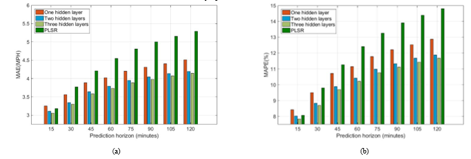
Figure 6. Speed prediction errors for I-66 in Virginia: (a) MAE; (b) MAPE.
As shown in Figure 6, the prediction errors worsened as the prediction horizon increased. At the 15-minute prediction horizon, PLSR was comparable to the neural network, as the correlation between the predictors and the responses was expected to be high, and the variability in the response could be explained using a linear model such as PLSR. However, as the prediction horizon increased, the relationship between the predictors and responses became nonlinear and the PLSR did not predict well. The neural network, on the other hand, had the ability to estimate a nonlinear function, and predicted well. It should also be noted that, as the number of hidden layers increased, the average errors decreased. In order to visually inspect differences among the four models, we plotted the average of the errors of all folds and estimated the 95% confidence interval, as shown in Figure 7.
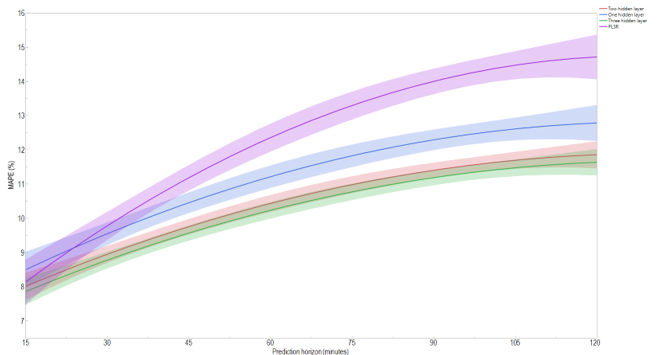
Figure 7. The speed MAPE and 95% confidence interval for the four developed models I-66 in Virginia).
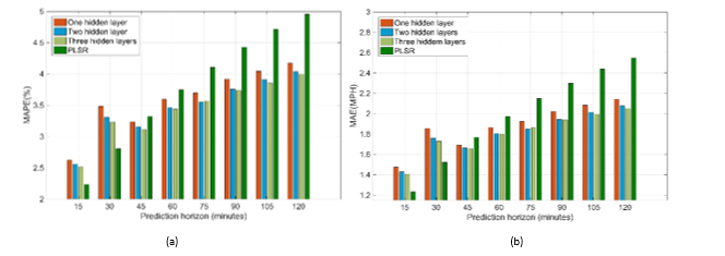
Figure 8. Speed prediction errors for I-15 in California; (a) MAPE; (b) MAE.
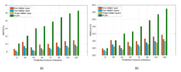
Figure 9. Flow prediction errors for I-15 in California; (a) MAPE; (b) MAE
As shown in Figure 7, at the 15-minute prediction horizon, all models are quite similar where their four confidence intervals intersect. At a larger prediction horizon, we can group the four models into three different groups. The first group includes the PLSR model; the second group includes the one-hidden-layer neural network model; the third group includes both the two- and three-hidden-layers neural network models. This figure suggests that the three-hidden-layers neural network is the best model, particularly at the 120-minute prediction horizon, as its confidence interval does not intersect with the one-hidden-layer neural network’s confidence interval.
7.3. I-15 Results
| In this section, we discuss the results of applying the proposed approach to a different dataset to predict the traffic states (speed/flow) for up to 120 minutes in the future for the studied stretch if I-15. We modeled the traffic state using shallow network models, the PLSR model, and deep network models. The prediction errors for both speed and flow at different prediction horizons are shown in Figure 8 and Figure 9, respectively. |
Figure 8 compares the shallow network and the two deep networks for the speed prediction, with the top panel showing the MAPE and the bottom panel showing the MAE. The PLSR model is shown as well for the sake of comparison. As the figure illustrates, the deep neural networks had smaller prediction errors compared to the shallow neural network. Moreover, the three-hidden-layers network did not remarkably reduce the average prediction error. However, the confidence intervals of the various models still need to be considered before deciding on a preferred model. Figure 8 also shows that at the 15-minute and 30-minute prediction horizon PLSR performed quite well, as there was high correlation between the input predictors and the responses. However, for the longer prediction horizons, neural networks returned better results than PLSR.
The flow prediction errors shown in Figure 9 indicate that the deep neural network had smaller prediction errors compared to the shallow neural network. Moreover, the three-hidden-layers network had the lowest prediction errors. Figure 9 also shows that the prediction errors for PLSR were the worst among all the models, especially for the long prediction horizons.
Figure 10 helps to differentiate between the models with close average errors. In this figure, we can visually inspect whether the four models are, in fact, different by plotting the average of the errors of all folds and estimating the 95% confidence interval.
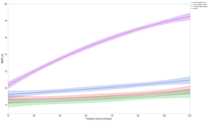
Figure 10. The flow MAPE and 95% confidence interval for the four developed models (I-15 in California).
As shown in Figure 10, the confidence intervals of the two- and three-hidden-layers neural networks intersect, indicating that they are not significantly different. However, the three-hidden-layers model is preferred because it does not intersect with the one-hidden-layer model at the 15-minute prediction horizon, and its confidence interval is far from that of the one-hidden-layer model’s confidence interval.
8. Conclusions and Future work
In this paper, we adopted discriminatively pre-trained deep neural networks to build a traffic state short-term prediction model. We compared a shallow neural network, a two-hidden-layers neural network, a three-hidden-layers neural network, and PLSR. The four models were used to predict traffic states for two different freeway road stretches. We used the divide-and-conquer approach to overcome the central processing unit time and memory requirements for long roadway stretches and large prediction horizons. The models were compared using MAE and MAPE measures. Experimental results showed that the three-hidden-layers neural network was the best model for traffic state short-term prediction and that PLSR was the worst among the four models. However, PLSR performed well at the 15-minute prediction horizon, as evidenced by its high correlation between the responses and predictors at that horizon.
Adding other factors, such as work zones and incident information, to the prediction models is planned in future studies. Adding these factors may explain some of the variability that cannot be accounted for using the current prediction models.
Note that the models proposed in this paper do not consider the response of travelers if they are receiving predicted traffic information disseminated by the agencies operating the network. Studying the interaction of informed travelers and including travelers’ responses as an input factor to the prediction models is an area for further work. Another area for future work is network-wide traffic prediction, for which models to predict the traffic on different roadway segments in a network will be developed. For network-wide prediction, we can make use of newly available technologies along with new big data techniques to integrate travel behavior and enhance traffic predictions. Moreover, online learning algorithms that continue to learn from each new incoming observation are needed to capture the dynamics of traffic patterns inside cities, which change over time.
- J. Young-Seon, B. Young-Ji, M. Mendonca Castro-Neto, and S. M. Easa, “Supervised Weighting-Online Learning Algorithm for Short-Term Traffic Flow Prediction,” Intelligent Transportation Systems, IEEE Transactions on, vol. 14, pp. 1700-1707, 2013.
- R. Arnott and K. Small, “The Economics of Traffic Congestion,” American Scientist, vol. 82, pp. 446-455, 1994.
- E. I. Vlahogianni, M. G. Karlaftis, and J. C. Golias, “Short-term traffic forecasting: Where we are and where we’re going,” Transportation Research Part C: Emerging Technologies, vol. 43, pp. 3-19, 2014.
- M. Elhenawy and H. Rakha, “Stretch-wide traffic state prediction using discriminatively pre-trained deep neural networks,” in 2016 IEEE 19th International Conference on Intelligent Transportation Systems (ITSC), 2016, pp. 1065-1070.
- M. S. Ahmed and A. R. Cook, Analysis of freeway traffic time-series data by using Box-Jenkins techniques, 1979.
- M. Van Der Voort, M. Dougherty, and S. Watson, “Combining Kohonen maps with ARIMA time series models to forecast traffic flow,” Transportation Research Part C: Emerging Technologies, vol. 4, pp. 307-318, 1996.
- S. Lee and D. Fambro, “Application of subset autoregressive integrated moving average model for short-term freeway traffic volume forecasting,” Transportation Research Record: Journal of the Transportation Research Board, pp. 179-188, 1999.
- B. M. Williams and L. A. Hoel, “Modeling and forecasting vehicular traffic flow as a seasonal ARIMA process: Theoretical basis and empirical results,” Journal of transportation engineering, vol. 129, pp. 664-672, 2003.
- G. A. Davis and N. L. Nihan, “Nonparametric Regression and Short-Term Freeway Traffic Forecasting,” Journal of Transportation Engineering, 1991.
- H. Sun, H. Liu, H. Xiao, R. He, and B. Ran, “Use of local linear regression model for short-term traffic forecasting,” Transportation Research Record: Journal of the Transportation Research Board, pp. 143-150, 2003.
- W. Zheng, D.-H. Lee, and Q. Shi, “Short-term freeway traffic flow prediction: Bayesian combined neural network approach,” Journal of transportation engineering, vol. 132, pp. 114-121, 2006.
- B. Park, C. Messer, and T. Urbanik II, “Short-term freeway traffic volume forecasting using radial basis function neural network,” Transportation Research Record: Journal of the Transportation Research Board, pp. 39-47, 1998.
- E. I. Vlahogianni, M. G. Karlaftis, and J. C. Golias, “Short-term traffic forecasting: Where we are and where we’re going,” Transportation Research Part C: Emerging Technologies, vol. 43, Part 1, pp. 3-19, 6// 2014.
- W. Huang, G. Song, H. Hong, and K. Xie, “Deep architecture for traffic flow prediction: Deep belief networks with multitask learning,” IEEE Transactions on Intelligent Transportation Systems, vol. 15, pp. 2191-2201, 2014.
- R. Yu, Y. Li, C. Shahabi, U. Demiryurek, and Y. Liu, “Deep Learning: A Generic Approach for Extreme Condition Traffic Forecasting.”
- N. G. Polson and V. O. Sokolov, “Deep learning for short-term traffic flow prediction,” Transportation Research Part C: Emerging Technologies, vol. 79, pp. 1-17, 6// 2017.
- Y. Lv, Y. Duan, W. Kang, Z. Li, and F.-Y. Wang, “Traffic flow prediction with big data: a deep learning approach,” IEEE Transactions on Intelligent Transportation Systems, vol. 16, pp. 865-873, 2015.
- X. Ma, Z. Dai, Z. He, and Y. Wang, “Learning Traffic as Images: A Deep Convolution Neural Network for Large-scale Transportation Network Speed Prediction,” arXiv preprint arXiv:1701.04245, 2017.
- J. Van Lint and C. Van Hinsbergen, “Short-term traffic and travel time prediction models,” Artificial Intelligence Applications to Critical Transportation Issues, vol. 22, 2012.
- D. E. Rumelhart, G. E. Hinton, and R. J. Williams, “Learning representations by back-propagating errors,” Cognitive modeling, vol. 5.
- D. Yu, L. Deng, F. T. B. Seide, and G. Li, “Discriminative pretraining of deep neural networks,” ed: Google Patents, 2011.
- H. Abdi, “Partial least square regression (PLS regression),” ed.
- S. Wold, A. Ruhe, H. Wold, and I. Dunn, W., “The Collinearity Problem in Linear Regression. The Partial Least Squares (PLS) Approach to Generalized Inverses,” SIAM Journal on Scientific and Statistical Computing, vol. 5, pp. 735-743, 1984.
- M. Elhenawy and H. Rakha, “Traffic Stream Speed Short-term Prediction using Machine Learning Techniques: I-66 Case Study,” presented at the the 95th Transportation Research Board Annual Meeting, Washington DC, 2016.