Power requirements and battery life measurement for wireless transmission between two nodes in different mediums
Power requirements and battery life measurement for wireless transmission between two nodes in different mediums
Volume 2, Issue 3, Page No 605-611, 2017
Author’s Name: Radouane Karli1, Abdellatif Bouchalkha2, a), Khalid Alhammadi1
View Affiliations
1Electrical Engineering Department, Khalifa University of Science and Technology, P.O. Box 127788, Abu Dhabi, United Arab Emirates
2Physics Department, Khalifa University of Science and Technology, P.O. Box 127788, Abu Dhabi, United Arab Emirates
a)Author to whom correspondence should be addressed. E-mail: abouchalkha@pi.ac.ae
Adv. Sci. Technol. Eng. Syst. J. 2(3), 605-611 (2017); ![]() DOI: 10.25046/aj020377
DOI: 10.25046/aj020377
Keywords: Wireless sensor, Battery life, Power consumption, ZigBee terminal

Export Citations
One of the most important roles of the wireless sensor networks (WSN) is to avoid wiring costs, be self-sustainable and be able to function for several years. However, due to the slow progress in battery technology, power continues to be a limited resource in wireless sensor communication and electric energy storage remains to be an important issue. On the other hand, if batteries must be replaced often, many remote sensing applications may become impractical. Therefore, batteries with long life on the order of several years are needed. This paper is an extension of work originally presented in The 5th International Conference on Electronic Devices, Systems and Applications to investigate further the power requirements for wireless data transfer between two nodes using batteries with different capacities (55 mAh, 550 mAh and 5500 mAh). In particular, the effect of a propagation medium such as air, distilled water and engine oil on the wireless communication inside a one meter long metallic pipe was investigated. Our first result shows a successful transmission of wireless signal through air, distilled water and oil medium with very low transmission losses. The second result shows that an increase in the battery capacity will increase the two-node wireless sensor operation time even in different propagation medium. This result can be used to determine the required battery capacity for extending the WSN operation time.
Received: 05 April 2017, Accepted: 12 May 2017, Published Online: 04 June 2017
1. Introduction
Pipelines in oil and gas industries constitute generally the most economical way to transport large quantities of oil, refined oil products or natural gas. The management of oil and gas transport in a pipeline is a challenging task with the rapid growth of the required length of pipelines. Challenges such as oil and gas leaks, pipeline corrosion, wax precipitation and environmental pollution are treated with highest priority in oil industries. Hence, the most common and important applications of WSN in oil industry are related to real-time monitoring of the production performance through process control, safety, and rigorous maintenance operations [1, 2].
Because of its crucial importance, the continuous operation of a WSN is essential and must be maintained at all time. The lifetime of a WSN can be defined as the life of the shortest living node in the network. However, depending on the application, the density of the network, and the possibilities of the network reconfiguration, it can also be defined as the life of some other (main or critical) nodes [2]. In order to prolong a WSN life, it is required to reduce the energy consumption of the nodes as much as possible [3].
However, for many important WSN applications, such energy option is not feasible, and specific power-management strategies are necessary for WSN nodes that are powered by non-rechargeable batteries. Energy consumption still remains one of the main obstacles to the development of WSN technology, especially in cases where long and reliable network operation is required [3].
To reduce the overall energy consumption of the network, one should use some power management (PM) techniques at the level of the sensing, communication, or processing unit. Another option is to consider using some energy harvesting techniques to extend the WSN operation time [5].In most cases once the WSN has been deployed, it is impossible to replace each and every battery present in the network after discharge. One important challenge in the design of a large WSN is energy efficiency where the design of a WSN should extend its life without sacrificing its reliability [4].
The main goal of this paper is to study the power consumption of a two-node wireless sensor communication for batteries with different capacities. Two experiments were considered for this study. The first one was the free space wireless communication in open air without metallic pipe and the second one was the wireless communication inside a metallic oil pipe acting as a waveguide. The measurement results showed that the data can be transmitted successfully through air inside a pipe with very low transmission loss. It was also shown that an increase in the battery capacity increases the two-node wireless sensor operation time. This result can be used to determine the required battery capacity for extending the wireless sensor system life time.
2. Linear Network
The architecture and proposed work for a general WSN may not be suitable for linear WSN applications such as monitoring pipelines. This requires a good review and a thorough study of the applications needing linear WSN to determine the specific design requirements for it.
There are several advantages for using linear alignment of nodes to provide protection and monitoring of linear topology such as oil, water, and gas pipelines. Some of these advantages include faster and less costly network deployment in addition to the ability to introduce flexible multi-hop routing which can overcome intermediate node failures.
In a linear distributed detection system, an initial sensor starts the detection process and make decisions then transmit both the data and the decisions to its neighbor as shown in Figure 1. Based on the received decisions from their predecessors, the succeeding sensors again form decisions and transmit them together with the data until the final sensor or gateway node is reached [6].
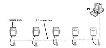
Figure 1. Linear structure of wireless sensor network
Since the pipeline network extends generally along a line, it is important for the network to be continuously connected to collect and transfer information from the sensor nodes distributed over the pipeline to the control station. It will also be required to transfer control commands to the actor and sensor nodes, which are often located inside the pipeline. The sensor network architectures generally used for reliable communication in pipeline systems are based on wired networks, wireless networks, or a combination of both. Typical applications [7, 8], include the case of sensors embedded in the outer surface of a pipeline. This linear sensor arrangement is the result of their linear topology.
Linear WSN is a special category of WSN where the nodes are placed in a linear form. Kevin et al., [9] gave two different definitions for the network topology model of a linear WSN. The first definition describes it as a connected non-cyclic diagram where each node has exactly one or two distinct neighbors. The two nodes with only one neighbor are referred to as the endpoints of the network. While the second definition presents it as a linear network topology containing N nodes where each node can communicate with other nodes up to a number M of hops [10, 11].
Lin et al., [12] have proposed an application of linear network in power transmission lines. In this case, they used a clustering algorithm to balance energy consumption and leverage hybrid media access control for monitoring the power transmission lines. This proposed technique makes the system complex to implement and less responsive. Akbar et al. [13], in their contribution to linear WSNs, proposed another technique. This consists of mobile sinks, and courier nodes that work underwater in a 3-D linear formation which minimizes energy consumption as well as accurately computing required routing information. Such 3-D linear system is, though accurate in routing, yet also too complex for real-time sensing and monitoring. This is especially the case for the implementation in mission critical applications such as pipeline monitoring.
Linear WSNs may be simplistic in topology but the decision of routing and deployment of nodes to conserve resources is not as simple as it may seem to be. A detailed hierarchical and topological classification and implementation of linear sensor networks is provided by Jawhar et al., and Liu et al., [14, 15]. In both cases it is difficult to implement in pipeline monitoring due to the surrounding harsh environment. Therefore, certain design requirements and research issues need to be addressed and investigated, given that few research papers have discussed the special requirements for linear WSN. These requirements have strong impact on the network performance.
On the other hand, extending the network lifetime is still a critical issue in many WSN cases. Different research groups have discussed this issue [16, 17], from the point of view of network power management software and protocol but not in terms of extending battery lifetime.
In this paper, we investigate the wireless transmission between two consecutive nodes to address the issues related to wireless communication in a linear WSN for long pipelines. The results of this work are very useful and can be extended to a multi-node linear system in the future.
3. Battery life
The two most important properties of a battery are its voltage level and its capacity (expressed in Ampere-hour, Ah) which represents the amount of energy stored in a battery. For an ideal battery, the voltage stays constant over time until the moment when it is completely discharged. Ideally, the battery’s capacity remains the same for any load. However, in a real situation, the voltage of a battery drops during the discharging phase and the effective capacity of a real battery is lower under a higher load. In this case, the high current draw decreases the battery capacity in a nonlinear behavior. In the case of an ideal battery, it would be easier to calculate the battery life L in the case of a constant load as follows [18, 19].![]()
Where C is the battery capacity and I is the load current.
The above simple relation does not hold for predicting the life of a real battery due to the various nonlinear effects neglected. A better and still simple approximation for the battery life calculation under constant load can be obtained from Peukert’s law. The later gives an expression for the capacity of a battery in terms of the rate of discharging. As a result, when the rate of discharging increases, the battery’s available capacity decreases. The formula for Peukert’s law can be expressed in different forms with the most common one used is shown below [19, 20]:![]()
Where;
L – The time, in hours, that the battery will last for a given rate of discharge.
H – The discharge time in hours.
C – The battery capacity in Amp-hours based on a specified discharge time.
I – Current in Amp.
k – Peukert exponent parameter which is a unique number for each battery.
4. Experimental setup
4.1. Wireless communication experiment
The wireless transmission experimental setup is shown in Figure 2. This setup consists of two wireless communication nodes using a fixed digital data set provided by an analog input voltage. The two nodes are standard ZigBee terminals powered by a lithium battery and communicating in the frequency range 2.4-2.5 GHz. The digital data is transmitted by the transmitter terminal and received by the receiver terminal which is interfaced to a PC through a National Instrument NI-ELVIS DAQ. An IP Modem Configure-F8114 and the SScom32E software were used for collecting data on the computer. The principle of operation is that the PC sends a command to the wireless ZigBee terminal F8114 connected through RS232 to a PC to communicate with wireless terminal F8914 and read its digital output data. The communication was established via simple dipole antennas to ensure unidirectional transmission between the two terminals. These directional antennas help reduce the effects of interference as well as extend the communication range between the two terminals. The dipole antennas have an impedance of 50Ω, a gain of 3 dB and a length of 125 mm. The data is then processed by the PC which is connected as shown in Figure 2.
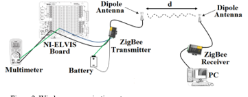
Figure 2. Wireless communication setup
The transmitter/receiver terminal uses the standard ZigBee communication protocol which is based on offset quadrature phase shift keying to transmit digital data [21]. The acquired data was in hexadecimal (HEX) format which was then converted to decimal (DEC) format. The corresponding value was then calculated, as described in the manual of the F8914 ZigBee Terminal.
For the study of the effect of a different medium on the wireless communication, we used a one meter long hollow metallic pipe made of iron as shown in Figures (3a) and (3b). We have also used the pipe as a waveguide for transmitting and receiving data wirelessly between the two dipole antennas driven by the two ZigBee terminals. The diameter and the thickness of the pipe were respectively 0.1 m and 0.003 m. The metallic pipe was placed between the two antennas and filled, alternatively, with distilled water or engine oil. The initially analog voltage data was transformed to ZigBee format and sent through these different mediums. The received values for air, distilled water, and oil mediums were recorded and compared to the transmitted values as will be shown later in Figure 5. The temperature was also kept constant at approximately 21±0.5 °C throughout the experiment.
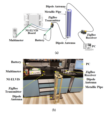
Figure 3. Experimental setup for wireless communication in a mettalic pipe as a diagram (a) and the actual laboratory setup (b).
4.2. Wireless node power requirement experiment
A common way of specifying the energy capacity of the wireless sensor is to provide the battery capacity as a function of elapsed time until it is fully discharged. The experimental setup used in this part is shown in Figure 4.
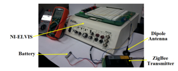
Figure 4. The battery voltage measurement setup
In this case, we maintained a good communication between the transmitter and receiver terminals but measured the load voltage of the battery connected to the transmitter as a function of the elapsed time. Three different batteries with different nominal capacities (55 mAh, 550 mAh and 5500 mAh) were used in our experiment. The power level of the transceivers was kept constant at 2.82 mW and the distance between the transmitter and receiver was fixed to either 1 m or 9 m.
The analog voltage value was converted to digital value first then transmitted wirelessly. The transmission was done continuously and after each transmission the battery voltage was recorded. The battery voltage level measurements were conducted at regular time intervals at the transmitter side. The communication between the emitter and the receiver was maintained and checked before each measurement to make sure it is successful.
5. Results and discussions
5.1. Two-nodes communication in different mediums
The results from the wireless communication experiment described earlier are shown in Figure 5. This experiment was conducted to establish wireless communication and compare the transmitted and received data between the two ZigBee terminals. From the figure it can be clearly seen that the voltage data was successfully transmitted through the three different mediums namely air, distilled water and engine oil with very low relative transmission losses. It can also be seen from Figure 5 that the wireless transmission is independent of the medium inside the pipe and the digital data was well received as expected and confirmed. This is a good confirmation that digital data transmission has experienced practically no losses even through a wide range of different propagation mediums such as air, distilled water and engine oil.
In oil wells, we are always monitoring the temperature and the pressure downhole as the most critical parameters. In general, the temperature is high and can easily reach 150 °C. In order to validate the above results, we have adjusted the previous experimental setup to transmit and receive real measured temperature data. The experimental setup used is shown in Figure 6 with wireless transmission through the 1 meter metallic pipe. In this case we have replaced the constant voltage value by a temperature sensor immerged in a variable temperature water bath. The temperature sensor used is a type K thermocouple (Chromel/Alumel) with a temperature range of -30 °C to 300 °C and an output voltage range of -6.4 mV to 54.9 mV.
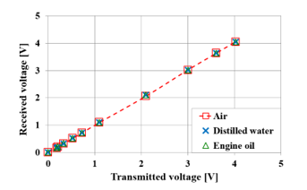
Figure 5. Comparison between the wirelessly transmitted and received voltage in a 1 meter long mettallic pipe for the different cases indicated.
The multimeter used is capable of measuring very low voltages across the two wires of the thermocouple as shown in Figure 6. The measured voltage was multiplied by the Seebeck constant to get the corresponding temperature [22]. This temperature was recorded as the input temperature. Since the thermocouple voltage was very low, it was fed to an AD620 instrumentation amplifier before the wireless transmittion and further processing. The received wireless signal is transformed back to temperature data and the results are shown in Figure 7.
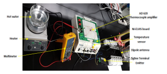
Figure 6. Wireless communication setup with Temperature sensor (Thermocouple K)
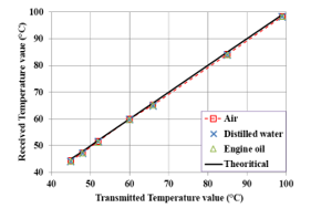
Figure 7. Comparison between the wirelessly transmitted and received temperature data in a 1 meter long mettallic pipe for the different cases indicated.
From Figure 7, it can be seen that the temperature data is successfully transmitted through air, distilled water and oil mediums with very low transmission loss. The maximum temperature limit of 100 oC is due to water evaporation temperature. Higher temperatures could be reached with other fluids such as oil if needed. From the graph we can estimate the error on the transmitted temperature to be about 0.7 % at 100 oC. This is very close to the expected K-type thermocouple uncertainty of 0.75 % at the same temperature. In comparison with the previous experiment, using constant voltage, where the error was negligible, we can conclude that the observed error in transmitting temperature data was mainly introduced by the thermocouple.
5.2. Battery life measurements
For the power requirement and battery life study, we consider the first results using a single battery B1 with a nominal capacity of 55 mAh. Figure 8 shows a comparison between the battery voltage level as a function of continuous wireless transmission time and distance between the nodes for the battery B1. The wireless transmission was conducted in air with and without a metallic pipe. Using the Terminal ZigBee powered by B1 with a distance of 1 m between the transmitter and receiver, we observed that the battery B1 had lasted for about 79 hours of continuous transmission. This is in good agreement with the value of 81 hours listed by the manufacturer. This is due to the special cutoff voltage of 8.8 V below which this battery is considered to be non-reliable.
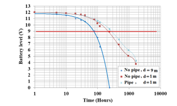
Figure 8. Comparison between the battery voltage level as a function of continuous wireless transmission time and distance between the nodes for the battery B1 with 55 mAh nominal capacity . The transmission was conducted in air with and without a metallic pipe.
It is also observed from Figure 8 that the distance between the nodes has an important effect on the data transmission. From the figure we can see that when the distance was changed from 9 m to 1 m without using the metallic pipe, the battery lasted for about 250 hours as opposed to 79 hours with the 9 m distance. This increases the battery life by a factor of 3. On the other hand, we noticed that using the metallic pipe as a cylindrical waveguide has also enhanced the battery life. This is due to the reduced attenuation effect from the open environment and the enhancement due to the waveguide effect making the transmission more directional. In this case according to Figure 8, the battery life measured for the wireless transmission in the metallic pipe under the same conditions was about 300 hours. Comparing the two results we can see that we have achieved a battery life enhancement of at least 20 % for this particular case. This is quite encouraging and will be investigated and optimized further in our future work.
In order to investigate further the battery life as a function of its capacity, we have chosen to conduct additional experiments with two other batteries B2 and B3 with higher nominal capacities of 550 mAh and 5500 mAh respectively. These experiments were conducted in open air for batteries B1, B2, and B3 as indicated in Table 1. The temperature of the environment was kept the same at around 21±0.5 °C and the distance between the transmitter and receiver was fixed to 9 m.
- Battery life measured at the cutoff voltage of 8.8V with B4 and B5 as indicated.
| Battery | Nominal capacity (Ah) | Battery life (years) |
| B1 | 0.055 | 0.009 |
| B2 | 0.55 | 0.02 |
| B3 | 5.5 | 0.16 |
| B4 [23] | 34 | 1 |
| B5 [24] | 700 | 20 |
The battery voltage level measurements at the wireless transmission node were recorded as a function of the continuous transmission time for the three different batteries B1, B2, and B3. The results are shown in Figure 9 with a cutoff voltage of 8.8 V as discussed earlier. From the graph we immediately notice that the battery life was longer for the higher capacity batteries as expected and confirmed by our measurements. We also notice that the measured battery voltage decreases more slowly for the batteries with larger capacities (B2 and B3) hence providing longer battery life according to the indicated cutoff voltage of 8.8 V.

Figure 9. Comparison between the battery voltage level as a function of continuous wireless transmission time for the batteries B1, B2, and B3 with nominal capacities 55, 550, and 5500 mAh respectively, in open air for a fixed distance of 9 m between the two nodes.
For the battery B2 with nominal capacity 550 mAh, it’s observed that the life of transmission is about twice greater than that of the battery B1 with nominal capacity 55 mAh. In addition, we found that the battery B2 lasted for about 170 hours of continuously transmitting data before reaching the minimum required cutoff voltage of 8.8V. For the third battery B3 with the nominal capacity of 5500 mAh, it was observed that after 1400 hours, the transmitter has consumed only 17 % of the battery’s capacity. In Table 1 we report the measured battery lives of the three different batteries obtained from Figure 9 at the cutoff voltage of 8.8 V.
The results in Table 1 were used to obtain the very useful graph shown in Figure 10. Note that the data for batteries B4 and B5 were obtained from the literature [23, 24]. The curve in Figure 10 is obtained from Equation (2) with I = 2.3 mA and k = 1.25 as the average value for most lead acid batteries [25]. Notice the good agreement between the measured and calculated battery life.
The graph in Figure 10 can be used to predict and estimate the remaining battery life at any moment in time during battery operation. This is quite useful for WSNs that require long-term operation with single batteries. As shown in Figure 10, the requirement for a specific battery life can also be determined. For example, a 15 years operation time can be reached with a 500 Ah capacity battery while a 10 years operation time requires a 320 Ah capacity battery as shown in the figure below. From the literature review and the available products in the market, these battery lifetimes are now accessible and currently used in certain applications. This, certainly, makes our predictions very useful to the users of these batteries. With our plot in Figure 10, one can estimate the remaining time for these long-life batteries and plan the required battery replacements.
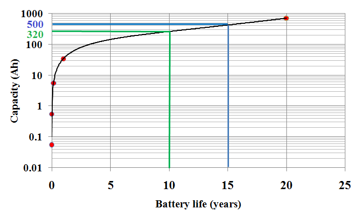
Figure 10. A plot of the different battery capacities as a function of their corresponding life. The line is a theretical curve fit as discussed in the text.
In summary, we conclude that the transmitting WSN nodes will perform well with long life batteries and small discharge time such as the case of the high capacity batteries. Also, from the measurement results, the digital data is successfully transmitted through air, distilled water, and engine oil mediums with very low transmission loss relative to air. We can conclude and confirm that the wireless transmission is well established and was not affected much by the two different mediums considered in our study which are distilled water and engine oil compared to air. We have also shown that the wireless transmission in a metallic pipe contributed at least 20 % more to the battery life of the wireless transmitter according to our current experimental setup. On the other hand, our results are more general and could be adapted to different types of wireless sensor networks to predict and monitor the required battery power.
6. Conclusion
In this paper, we have presented the study of a two-node wireless communication considering both the medium of propagation and the power requirements. The two terminals used were ZigBee terminals with dipole antennas placed at the ends of a metallic pipe filled with air, distilled water or engine oil. Our experimental results showed that efficient communication between the two wireless nodes was well established in air, distilled water and engine oil at the standard communication band of 2.4-2.5 GHz.
We have also presented the wireless sensor power requirement study and the required battery life for sustained wireless communication of a continuously transmitting node. The study of the battery life allowed us to estimate the required battery capacity for a specific long-term wireless sensor operation. For example, for a 15 years operation time one needs a battery of at least 500 Ah capacity. This estimation can be conducted for any specific wireless node power requirement. This study enables predictions concerning the service life for long-term use of batteries. The experimental results showed that the rate of energy discharge varies from one battery to another and can be quite long for large capacity batteries. When the battery capacity is large, it ensures good life of the wireless sensor transmission and the WSN.
This work is the first phase of a big project that will be continued and implemented. We would expect to extend our work in the future to include other components such as temperature sensors, pressure sensors, gateways and other models for wireless sensor networks. This will be mainly targeting the oil pipeline monitoring for addressing specific flow assurance challenges. We will also investigate further the 20 % battery life enhancement observed in the case of the guided wave conditions that we setup in the metallic pipe.
Acknowledgment
This work was funded through the Project No. RDProj.041-FA by Abu Dhabi National Oil Company (ADNOC), R&D, Abu Dhabi, United Arab Emirates (UAE).
- R. Karli, A. Bouchalkha and K. Alhammadi, “Power consumption and battery life study of a two-node wireless sensor system”, The 5th International Conference on Electronic Devices, Systems and Applications, December 6-8, Ras Al Khaimah, UAE, 2016.
- M. A. Akkaş, R. Sokullu and A. Balcı, ”Wireless Sensor Networks in Oil Pipeline Systems Using Electromagnetic Waves”, The 9th International Conference on Electrical and Electronics Engineering (ELECO), 2015.
- A. Moschitta and I. Neri, Power consumption Assessment in Wireless Sensor Networks, ICT – Energy – Concepts Towards Zero – Power Information and Communication Technology: Dr. Giorgos Fagas (Ed.), InTech, DOI: 10.5772/57201, 2014.
- Y. Chen and Q. Zhao, “On the Life of Wireless Sensor Networks”, IEEE Communications Letters, Vol. 9, Issue 11, pp. 976–978, 2005.
- I. Dietrich and F. Dressler, “On the life of wireless sensor networks”, ACM Transactions on Sensor Networks, Vol. 5, issue 1, pp. 1-38, 2009.
- Gernot Fabeck, Rudolf Mathar, “Optimization of Linear Wireless Sensor Networks for Serial Distributed Detection Applications”. Vehicular Technology Conference (VTC 2010-Spring), IEEE 71st, 2010.
- S. Yoon, W. Ye, J. Heidemann, B. Littlefield, and C. Shahabi, “SWATS: Wireless sensor networks for steamflood and waterflood pipeline monitoring,” Netw. IEEE, Vol. 25, issue 1, pp. 50–56, 2011.
- T. T.-Te Lai, W.-J. Chen, K.-H. Li, P. Huang, and H.-H. Chu, “Triopusnet: Automating wireless sensor network deployment and replacement in pipeline monitoring,” ACM/IEEE 11th International Conference on Information Processing in Sensor Networks (IPSN), pp. 61–71, 2012.
- K. J. Henry, D.R. Stinson, “Resilient aggregation in simple linear sensor networks”, IACR, Cryptology ePrint Archive, 2014.
- S. Ali, S. Bin Qaisar and E. A. Felemban, “Dimensioning of linear and hierarchical wireless sensor networks for infrastructure monitoring with enhanced reliability”, KSII Transactions on internet and information systems, Vol. 8, No. 9, Sep. 2014.
- Changqing Xia, Wei Liu, and Qingxu Deng, “Cost Minimization of Wireless Sensor Networks with Unlimited-lifetime Energy for Monitoring Oil Pipelines”, IEEE/CAA Journal of Automatia Sinica, Vol. 2, No. 3, 2015.
- J. Lin, B. Zhu, P. Zeng, W. Liang, H. Yu, and Y. Xiao, “Monitoring power transmission lines using a wireless sensor network,” Wireless Commun. Mobile Comput., Vol. 15, No. 14, pp. 1799—1821, 2015.
- M. Akbar, N. Javaid 1, A. Hussain Khan, M. Imran, M. Shoaib, and A. Vasilakoset al., “Efficient data gathering in 3D linear underwater wireless sensor networks using sink mobility,” Sensors, Vol. 16, No. 3, pp. 404–431, 2016.
- I. Jawhar and N. Mohamed, “A hierarchical and topological classification of linear sensor networks,” in Proc. IEEE Symp. Wireless Telecomm., pp. 1–8, 2009.
- Y. Liu, J. Feng, O. Simeone, J. Tang, A. M. Haimovich and M. C. Zhou, “Topology discovery for linear wireless networks with application to train backbone inauguration,” IEEE Transactions on Intelli. Transp. Syst., Vol. 17, No. 8, pp. 2159–2170, 2016.
- Xia C Q, Guan N, Deng Q X, Yi W. Maximizing lifetime of threedimensional corona-based wireless sensor networks. International Journal of Distributed Sensor Networks, Article ID 149416, 2014.
- Keskin M E, Altinel K, Aras N, Ersoy C. Wireless sensor network lifetime maximization by optimal sensor deployment, activity scheduling, data routing and sink mobility. Ad Hoc Networks, 17, pp. 18-36, 2014.
- M. R. Jongerden and B. R. Haverkort, “Which battery model to use?” IET, Vol. 3, No. 6, pp. 445-457, 2009.
- D. Linden and T. B. Reddy, Handbook of Batteries, 3rd Edition, McGraw-Hill, ISBN 0-07-135978-8, 3-12, 2002.
- G. Wu, R. Lu, C. Zhu and C. C. Chan, “Apply a Piece-wise Peukert’s Equation with temperature correction factor to NIMH battery state of charge estimation” Journal of Asian Electric Vehicles, Vol. 8, No. 2, pp. 1419–1423, 2010.
- Ha H. Nguyen and Ed Shwedyk, “A First Course in Digital Communications”, Cambridge university Press, ISBN 0521876133, 2009.
- Arman Molkim, “Simple Demonstration of the Seebeck Effect”, Science Education Review, Vol. 9, No. 3, pp. 103–107, 2010.
- LTC batteries, SL-2790/S Sandard, catalogue No. 11 2 17901 00, Tadiran Batteries GmbH.
- Thomas Dittrich, Chen Menachem, Herzel Yamin and Lou Adams, “Lithium Batteries for Wireless Sensor Networks”, Tadiran Batteries GmbH.
- D. Doerffel and S. Abu Sharkh, “A critical review of using the Peukert equation for determining the remaining capacity of lead-acid and lithium-ion batteries”, Journal of Power Sources, Vol. 155, No. 2, pp. 395–400, 2006.