Homemade array of surface coils implementation for small animal magnetic resonance imaging
Homemade array of surface coils implementation for small animal magnetic resonance imaging
Volume 2, Issue 3, Page No 532-539, 2017
Author’s Name: Fernando Yepes-Calderon1, a), Olivier Beuf2
View Affiliations
1Children’s Hospital Los Angeles, Neurosurgery Division; 4650 Sunset Blvd, Los Angeles, CA 90027, USA
2Universite de Lyon, CREATIS INSA-Lyon; Villeurbanne 69100, France
a)Author to whom correspondence should be addressed. E-mail: fernandoyepesc@gmail.com
Adv. Sci. Technol. Eng. Syst. J. 2(3), 532-539 (2017); ![]() DOI: 10.25046/aj020368
DOI: 10.25046/aj020368
Keywords: MRI, Small Animal, Receptor antennas, Mutual induction, Parallelization

Export Citations
Small animal modeling is an exciting research field where human pathogenic frameworks can be replicated in a controlled environment. Accurate Imaging is in high demand when modeling abnormalities and, magnetic resonance imaging plays a vital role due to its demonstrated lowest intrusion when compared with other imaging methods. However, the required high-resolution yields low-quality images and often, critical events are masked. In this manuscript, we improve the images in small animal frameworks by modifying the reception coils to parallelize the readings and by dealing with the mutual induction produced at the dimensions required for the studied subjects.
Received: 06 April 2017, Accepted: 12 May 2017, Published Online: 01 June 2017
1 Introduction
Magnetic Resonance Imaging (MRI) has become a ubiquitous tool in imaging research and clinical radiology due to its capacity to provide non-invasive, in-vivo images, both in humans and in animal models. Small animals are widely used in disease research as their size make them particularly easy to manipulate; however, MR imaging is also significantly more challenging in smaller structures. The trade-off between the spatial resolution and signal-to-noise ratio (SNR) becomes exceptionally important when scanning small volumes.
Despite improvements in high field magnet technology at 7T and beyond, several factors reduce image quality so that larger fields may not mean better images. In particular, T1 lengthening, T2 shortening, and chemical shifts artifacts account for lowering the image quality well below theoretical expectations in high field magnets [1]. In contrast, parallel acquisitions improve image quality while avoiding all of these issues [2]. Simultaneous acquisitions require single receptors to be split into two or more simple loops while maintaining the field of view (FOV). This dimensional reduction is, initially, convenient because smaller receptors provide higher sensitivity and field stability [2], [3]. Nevertheless, when two or more coils share a common space, theirmutual inductance (MI) [4] deteriorates the receptor characteristics of the coils to the point where images can not be produced.
Here we present strategies to increase the quality of MRI images in surface coils and to minimize the deteriorating effects of MI. The first involves a shared capacitor placed between adjacent loops that counteracts the rising MI at Larmor frequency (Fr ). A second strategy, accomplished with pre-amplifiers, consists in diminishing the electrons’ flow among the receptors, so the factor Ldi dt is reduced; therefore, MI declines as well. This last strategy is intended to deal with high order MI, which is likely to be an issue when reading parallelization involves more than two channels.
We also determine the effect of implementing these MI reducing strategies both, independently and combined by analyzing the SNR, the field stability and the sensitivity of the coils for the images produced.
2 State-of-the-art technology
The concept of reducing the coils’ area to produce more efficient receptors, which was introduced by Roemer in [2] is both, attractive and challenging. It has numerous technical advantages, such as the possibility of creating adaptable devices that can fit almost any volume, while maintaining modularity [5]. A reasonable attempt at using multiple surface coils was presented by the Petals Project [6]. In that work, the receptor device consisted of a crown of resonant loops for hydrogen nuclei magnetized at 1.5T. The authors elegantly avoided near (first order) and next to near (higher order) MI by placing a gap between receptors. One drawback of this approach is that images of the brain presented not only progressive in-depth deterioration, but also fuzzy regions between the ”petals.” In spite of these issues, the Petals Project work showed the validity of the multiple coil approach and provided an important step towards applicability, while demonstrating the flexibility of the device.
The reception capabilities of the coil circuitry are not only dependent on its electrical length, but also on its geometrical configuration. For example, in [7], planar devices were build for which proper decoupling was enforced at the cost of reduced flexibility. In humans, [5] designed an interfacing box that allowed to connect up to 16 coils with different shapes, generating images with good contrast, though with an FOV of 200cm2. Notwithstanding these high dimensions (a surface coil of 200cm2 is too big for scanning a rat or mice), the circuitry is stable due to the larger values of its reactive components. The dynamically adaptable tuning-and-matching box is feasible due to the relatively big size of humans, but its implementation with smaller devices has various drawbacks associated with the electrical length of connectors and their dependence on frequency. The problem of making coils invisible to each other in an array disposition is well depicted in [8], where the authors proposed a geometrical method by placing a butterfly coil in parallel with a loop component. Through this configuration, a 90◦ combination of signals isolated the array from second and superior order MI while critical overlapping accounted for first order MI. This implementation was accomplished by arranging commercial coils to suit the quadrature configuration and presents and alternative to the low impedance preamplifiers in Roemer’s small coil strategy [2]. Yet in [7], the authors stated one more motivation to implement smaller receptors. Apart from offering better field stability and more in deep tissue penetration, its implementation, due to the inherent FOV reduction and the necessity to recover it, forces the use of parallel imaging (PI), which in turn reduces acquisition time. Following this initiative, several other authors looked into the so-called array coil. In particular, in [9] and [10], human array coils were designed for PI implementation, which allowed the use of standard reconstruction methods such as Simultaneous Acquisition of Spatial Harmonics (SMASH) [11], Sensitivity Encoding (SENSE) [12], Generalized Auto-Calibrating Partially Parallel Acquisitions (GRAPPA) [13], [14] and their improvements or variations [15]. The idea is that a complete positioning axis can go from being encoded in a voxel-by-voxel fashion to being wholly or partially encoded in one TR depending on the length of the array and its relative dimensions about the subject being scanned. Consequently, the acquisition time is dramatically reduced.
For small animal imaging, the reduced size of the subjects imposes new challenges. For example, circuits may be too long or of unsuitable geometries.
Also, the dynamic components are smaller, making the circuitry less stable. In spite of these issues, array coils have been used for specific applications like in [16], where rodents are scanned at ultra-high magnetic fields. In this case, the images are read with a three-channeled device, but each channel has been built to detect a different element’s nuclei, and therefore, their resonance frequency is different. Thus, MI is minimized by the selectiveness of the receptors. In one more small animal implementation, a novel imaging method capable of detecting redox-status, oxygenation and free radicals has also been introduced as a functional MRI strategy. This has been called Electron Parametric Resonance (EPR) [17], and is implemented through a 4-channel coil array. Here, the receptors are activated sequentially; thus, there is no need of MI decoupling methods.
The work presented here is a step toward creating operative MRI surface coils. Our model consists of a single loop coil that is replicated to build a two elements receptor. Once the coils share the same space, the MI affects the reading. Two strategies for avoiding MI are implemented. The first consists of a shared capacitor that counteracts the MI by resonating at the working frequency with the inductive effect; therefore, turning the induction circuit in a purely resistive device. The second strategy consists of adding a low impedance pre-amplifier to the parallel channels, so the read signals are transported as voltage instead of current; consequently, the induction principle of Faraday is minimized.
The design suits the small animal dimensions. At these sizes and working frequencies, one faces instability of the electronic components, high influence of geometry and the fact that even a simple cable can become any active component – a capacitor or an inductor – therefore making of the resonance condition, a moving target.
3 Materials and Methods
All experiments presented here were performed using a Biospec 4.7T MRI Bruker system, setup to enable the surface coil mode and PI. This system is usually sold with volumetric coils as the original acquisition device; Although, these antennas may be changed to suit animal dimensions. The software can be adapted to either use volumetric coils that have the emitter and the receptor on the same device or to use two different devices; thus making of the surface coil, the receptor device. Under the surface coil scheme, the emitter can be any of the individual coil sets provided by the manufacturer.
The new devices are Printed Card Board (PCB) loops designed using the Eagle software [18]. The associated circuitry was created following the procedure depicted in [19]. The devices were simulated and tested individually in a network analyzer (Agilent – E5062A-275) before coupling them to the MRI scanner. All coils were matched at 50Ω and tuned at
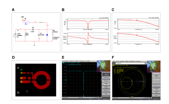 Figure 1: MRI single surface coil fabrication. A. Schematic of the circuit. B. Simulation of magnitude and phase responses of the circuit in A. C. The output of the circuit in magnitude and phase when the decoupling pin diode (line 4 in A) is on, providing protection to the coil against MRI RF pulsation. D. PCB of the real single surface coil. E. The amplitude response of the designed circuit read in the network analyzer around frequency Fr. F. Zero Index of signal reflexion in the coil’s terminals depicted in a Smith diagram. The PCB in D, when mounted, is used to create the displays in panels E and F (see upper right corner of these two panels).
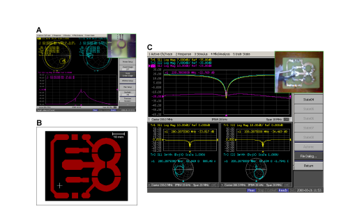 Figure 2: Two loops MRI receptor. A. Reduced emission/reception capabilities due to MI (see loops in the upper right panel). B PCB of the two-elements coil. C. Proof-of-concept: two coils magnetically separated by a shared capacitor. Here, the loops behave as if they were single devices, similar to the scheme in figure 1-E.
The Smith diagrams show perfect matching and tuning in both loops
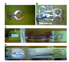 Figure 3: A.Single loop device (SD) B. Two elements device (DD), using a shared capacitor for decoupling. C. Single loop device with pre-amplifier (SDWP) connected trough a cable. D. Two elements device with pre-amplifier (DDWP), using a shared capacitor and connected trough a cable.
(fr) which corresponds to 200.3 MHz, as dictated by hydrogen spins magnetized at 4.7T. The different devices that we tested consist of:
- SD → A single-loop coil, 15mm in diameter.
- DD → A two-elements coil with shared capacitor, 2x15mm in diameter.
- SDWP → A single-loop coil with low impedance amplifier, 15mm in diameter.
- DDWP → A two-elements coil with shared capacitor and pre-amplifiers, 2x15mm in diameter.
Figures 1 and 2 show the circuit design and simulation, as well as evidence of accurate tuning and matched properties for the SD and DD devices.
3.1 Reducing di/dt. The low-impedance pre-amplifier
The role of the low-impedance pre-amplifier is to reduce current flow trough the coils’ terminals; therefore, the MI is also lowered [20]. The objective of this strategy is to obtain a circuit that has a high impedance on the coil side and, simultaneously, a low impedance at the preamplifier’s terminals at frequency Fr. In order to accomplish this, the λ/4 concept described in [21] is used. Briefly, the λ/4 length happens to be the distance at which a coaxial cable like the one used for transmission inside the scanner, becomes the desired device (high impedance on one side, a low impedance in the opposite). Using the network analyzer and the Smith diagram, this length was found to be 21cms.
The λ/4 cable is then plugged-in to the terminals of the two devices already created. Figure 3 shows the final setup of the receptors.
The images are created on phantoms using T1 contrast and multi-slice-multi-echo sequence (MSMEpvm) [22]. The repetition and echo times (TR and TE) are 261.4 and 10.7 ms, respectively, with a flip angle of 180◦; isometric in-plane resolution of 0.136mm; slice thickness of 2mm; 35x35mm2 FOV; 256x265 matrix, 8 slices for single loop coils, and 16 for the twoelements ones. The acquisition time is kept at 3.06 minutes for all experiments. The phantom for single loops coils consists of a circular syringe 15mm in diameter, while the two-elements devices scanned a syringe of 30 mm in diameter. Both phantoms contain a mix of water, salt (4.5%) and gadolinium. We performed six acquisitions per device. The five most centered slices in the volume of interest of each experiment are used to compute statistical comparisons (see Table 1).
3.2 Measures of coils performance and comparisons mechanisms
Measures of SNR, field stability, and visual depth were gathered from the acquired images. The SNR is obtained in the time-domain as the ratio between the signal – high-intensity pixels arranged in a circular fashion – and the standard deviation of the intensities in the background. The field stability was characterized by the horizontal profile while visual depth was obtained from the vertical profiles, where amplitude and signal decay are separately analyzed. All measures were done in axial views. A Shapiro-Wilk test was run over the data to determine the normality of the distribution. T-tests were performed on all the normally distributed data. However, the horizontal and vertical (amplitude and decay) profiles resulted in not normally distributed data, so we used the MannWhitney U test for statistical comparisons. Table 1 summarizes the factors we analyzed, the statistical tests, the comparisons we used and the questions that we addressed with each test. Statistical significance is assessed using a threshold of p = 0.05. All the statistics mentioned above were computed with SPSS.
4 Results
This section presents the results of applying the measurements described in Subsection 3.2. Color coding and labeling are provided; moreover, the colors are coherent throughout all sections for a fast association between the result and the device under test. The leftmost panel in each figure shows the regions where the data were gathered.
4.1 SNR comparisons
For each device, the SNR was measured by taking as signal a disk in the high-intensity region at the center of the image and, as noise, the standard deviation of intensities in the rest of the FOV.
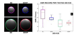 Figure 4: Panel A. Single loop devices exhibit a higher image quality as measured by the SNR, nevertheless it is in this group (the single devices) where the preamplifier generates the largest gap in quality when comparing with its counterpart (SDWP). Remarkably, in both, single and double device groups, the use of the pre-amplifier reduces the noise dispersion. In the double-loop devices, the pre-amplifier does not modify the SNR.
No statistical differences in SNR were found (t(14)=1.47, p=0.16) between SD (x = 28.54±7.95) and SDWP (x = 23.44±3.48). For the DD devices, the average for DD and DDWP were respectively 19.05±6.35 and 18.99±1.64. They were not statistically different from each other (t(10)=0.024, p=0.98).
4.2 Field stability
A Gaussian filter is applied to the original profile aiming to recover its low-frequency component, which is in turn, a measure of the field stability. The cutoff frequency is automatically extracted from the properties of the given profile by truncating its Fourier spectrum at 90% of the spectral energy content. Posteriorly, a homemade program iteratively looks for a polynomial that fits the filtered signal. The algorithm stops when the correlation coefficient reaches the value of 0.995, then, the index of the fitted polynomial is saved for each profile. In SD devices, the fitted polynomial found from 3 to 7 constraints, with an average of 5 for the two included devices. In DD devices, there is a natural increment of the tortuosity due to the boundary created by the two channels. The asymmetry in the profile was a constant in all the tested devices; we hypothesize this is due to a difference in the copper deposition in the construction process.
4.3 Visual depth
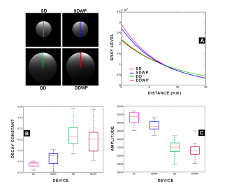 Figure 6: Comparison of vertical profiles. The vertical profile can be compared among all tested devices since the composition in the phantoms is the same for all devices regardless of their size. Panel A shows the decay while penetrating the phantom in all devices. Panels B and C show the data distribution in decay and amplitude respectively for each tested device.
In the single loop device, the use of the preamplifier reduces the dispersion in the decay constant. Nonetheless, the mean value for this decay is
faster when the pre-amplifier is used. Both versions of
the two elements loop allow the system to decay more slowly compared with their single loop counterparts. The amplitude in SD and DD devices can not be compared due to the loss of quality factor evidenced when looking at Figures 1-E and 2-C. Additionally, the amplitude and the decay constant can be separated for this specific analysis since the peak amplitude of the signal depends solely on construction specifications while the signal decay is a function of recruited spins. Considering that the phantom contains the same solution for all tested devices, the signal decay can be use for comparing all built devices, but an amplitude comparison will be only fair if done intra-group.
Table 1: Questions addressed and statistical tests performed
| Factor | Test | Comparisons | Addressed question |
| SNR | T-test | (SD-SDWP) | Is the quality of the images affected by addition of the pre-amplifier? |
| SNR | T-test | (DD-DDWP) | Is the quality of the images affected when the pre-amp and the shared capacitor are in place? |
| Horizontal | MWU | (SD-SDWP) | Is the field homogeneity affected by the pre-amp? |
| Horizontal | MWU | (DD-DDWP) | Is the field homogeneity affected by the pre-amp if another MI avoiding strategy is used? |
| Amplitude | MWU | (SD-SDWP) | Is the amplitude of the acquisitions affected by the use of the pre-amp? |
| Amplitude | MWU | (DD-DDWP) | Is the amplitude of the acquisitions affected when the pre-amp and the shared capacitor are in place? |
| Decay | MWU | (SD-SDWP) | Is the use of the pre-amp affecting the visual depth? |
| Decay | MWU | (DD-DDWP) | Is the visual depth affected when pre-amp and the shared capacitor are in place? |
| Decay | MWU | (SD-DD) | Is the visual depth of the coils increased when the inner diameter of the device decreases? |
| Decay | MWU | (SDWP-DDWP) | Is visual decay affected when two MI avoiding strategies are implemented together? |
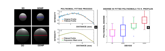 Figure 5: Panel A. Summary of the procedure for the horizontal profiles. Panel B. Distribution in tortuosity of the horizontal profiles in each device, measured as the degree of the first polynomial adjusted at 0.995 index of correlation
Table 2: Results of statistical tests. * experiments where statistical differences are found
| Factor | Test | Comparisons | p-value | Statistic values | |
| SNR | T-test | (SD-SDWP) | (28.54±7.95),(23.44±3.48) | 0.16 | t=1.47 df=14 |
| SNR | T-test | (DD-DDWP) | (19.05±6.35),(18.99±1.64) | 0.97 | t=0.03 df=9 |
| Horizontal | MWU | (SD-SDWP) | (4.46±0.86),(4.76±1.33) | 0.41 | U= 396.50, Z=0.83 |
| Horizontal | MWU | (DD-DDWP) | (5.63±0.85),(6.5±0.97) | 0.0013* | U=247.50, Z=3.22 |
| Amplitude | MWU | (SD-SDWP) | (29096.36±1586.54),(27222±1315.57) | 0.001* | U=731.00, Z=-4.15 |
| Amplitude | MWU | (DD-DDWP) | (21971.4±1665.32),(21526.8±2375.99) | 0.1421 | U=550.00, Z=-1.48 |
| Decay | MWU | (SD-SDWP) | (−14.24±0.002),(−0.1366±0.005) | 0.0002* | U=193.50, Z=-3.79 |
| Decay | MWU | (DD-DDWP) | (−0.115±0.010),(−0.119±0.012) | 0.224 | U=533.00, Z=1.23 |
| Decay | MWU | (SD-DD) | (29096.36±1586.54),(21971.4±1665.32) | 0.001* | U=0.00, Z=6.65 |
| Decay | MWU | (SDWP-DDWP) | (27222±1315.57),(21526.8±2375.99) | 0.001* | U=109.50, Z=5.03 |
The built devices are capable of MRI imaging, that should be and indubitable statement at this point due to the vast evidence presented with the Smith diagrams in Figures 1 and 2. However, we show in Figure 7, proof of the images that may be acquired with the sort of surface receptors designed and built along the development of the experiments that support the statements in this manuscript.
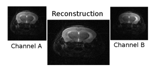 Figure 7: Image of mice’s brain using a DDWP device
5 Discussion
Our hypothesis is that the DD devices behave similarly to the SD devices when MI is diminished or avoided, and this claim is validated in those experiments with no statistical differences. Hence, we focus the discussion on those trials that resulted in statistical differences, and on their practical implications. Refer to the entries labeled with * in Table 2.
A significant difference (U= 247.50, Z=3.22, p=0.001) is found between DD (x = 5.63 ± 0.85) and DDWP (x = 6.5 ± 0.97). The mean rank of DD was 32.25, and that of DDWP was 23.75. These results have a low practical impact since the horizontal dynamics can be controlled by software reconstruction. In this case, we used a geometrically driven algorithm to merge the two channels, but customized setups can be implemented to optimize the smoothness of the boundary [1]. Nevertheless, the high degree of the fitted polynomials, even in the single loop devices, suggest a lack of uniformity in the copper deposition of our devices. This is observable in figure 5-A, which belongs to the SD device. A perfectly build coil within a flat B0 field should have a profile that can be modeled with a two-degree polynomial.
In the amplitude analysis, there was a significant difference (p≤ 0.05) between SD (x = 29096.36±1586.54) and SDWP (x = 27222 ± 1315.57) (U= 731.00, p=0.0013). The mean rank of SD was 21.13, and the mean rank of SDWP was 39.87, suggesting that the use of the pre-amplifier negatively affected the reading capabilities of the device; However, the practical implications of this finding are null, since it affects the single loop devices where the pre-amplifier does not introduce any added value. The pre-amplifier was connected to a single loop device with the purpose of creating a fair counterpart to compare the outcomes of the DDWP device. More importantly, the pre-amplifier in DD devices does not result in statistical differences, a fact of high relevance towards applicability.
In the decay analysis, there is a significant difference (U = 193.50,p < 0.001) between SD (x = −14.24 ± 0.002) and SDWP (x = −0.1366 ± 0.005). The mean rank of SD decay is 21.95, and the mean rank of SDWP decay is 39.05. There is no significant difference (U = 533.00,p = 0.22) between DD (x = −0.115 ± 0.010) and DDWP (x = −0.119 ± 0.012). The mean rank of DD decay is 33.27, and that of DDWP decay is 27.73. These results imply that visual depth is affected by the pre-amplifier in the group of devices that are not affected by the MI. In contrast, the pre-amplifiers do not have a significant influence on the signal in DD devices, where MI exists. There was also a significant difference (U = 0.00,p < 0.00) between SD (x = −14.24 ± 0.002) and DD (x = −0.115 ± 0.010). The mean rank of SD decay was 45.50, and the mean rank of DD decay was
15.50. The reduction of the diameter in the coils improves the reading capabilities of these devices. There was a significant difference (p≤ 0.05) between SSWP (x = −0.1366±0.005) and DDWP (x = −0.119±0.012); U = 109.50,p < 0.001. The mean rank of SDWP decay was 41.85, and the mean rank of DDWP decay was 19.15, which suggest that both strategies can be used together without affecting the quality of the images.
6 Conclusions
The small animal modeling field would be greatly benefited if accuracy in the visual monitoring methods is improved. An imaging setup with better outcomes would also yield more robust results, and the derived conclusions would be less questionable. In the end, animal experimentation is the only means that humanity has to test and study the progression of diseases and to anticipate the outcomes of procedures in living subjects. In this manuscript, we demonstrated that a better MRI receptor device, suitable to work at small animal dimensions is feasible. To this purpose, we implemented MI avoiding strategies and proved that they could be used together without significantly affecting the signal quality while enabling a more efficient use of the scanning time.
- O. Beuf, F. Jaillon, and H. Saint-Jalmes, “Smallanimal MRI: Signal-to-noise ratio comparison at 7 and 1.5 T with multiple-animal acquisition strategies,” Magn Reson Mater Phy, vol. 19, pp. 202 – 208, 2006.
- P. Roemer, W. Endelstein, C. Hayes, S. Souza, and O. Mueller, “The NMR Phased Array,” Magenetic Resonance In Medicine, no. 16, pp. 192–225, 1990.
- D. Gareis, T. Wichmann, T. Lanz, G. Melkus, M. Horn, and P. M. Jakob, “Mouse MRI using phased-array coils,” NMR Biomed., vol. 20, pp. 326 – 334, 2007.
- K. Sahay and S. Pathak, Basic Concepts Of Electrical Engineering. New Age International, 2006.
- N. D. Zanche, J. A. Massner, C. Leussler, and K. P. Pruessmann, “Modular design of receiver coil arrays,” NMR Biomed., vol. 5, 2007.
- S. S. Hidalgo, R. Rojas, and F. A. Barrios, “A petal resonator volume coil for MR neuroimaging,” Revista Mexicana de Fisica, vol. 52, no. 3, pp. 272 – 277, 2006.
- R. F. Lee, C. R. Westgate, R. G. Weiss, D. C. Newman, and P. A. Bottomley, “Planar strip array. PSA,” Magnetic Resonance in Medicine, vol. 45, no. 1, pp. 673 – 683, 2001.
- C. C. Guclu, E. Boskamp, T. Zheng, R. Becerra, and L. Blawat Journal of Magnetic Resonance Imaging, vol. 19, pp. 255 – 258, 2004.
- B. Keil and L. L. Wald, “Massively parallel MRI detector arrays,” Journal of Magnetic Resonance, vol. 229, pp. 75 – 89, 2013.
- C. Qian, G. Zabow, and A. Koretsky, “Engineering novel detectors and sensors for MRI,” Journal of Magnetic Resonance, vol. 229, pp. 67 – 74, 2013.
- D. Sodickson and W. Manning, “Simultaneous acquisition of spatial harmonics (SMASH): fast imaging with radiofrequency coil arrays.,” Magnetic Resonance in Medicine, vol. 38, pp. 591–603, 1997.
- K. P. Pruessmann, M. Weiger, M. B. Scheidegger, and P. Boesiger, “SENSE: Sensitivity Encoding for Fast MRI,” Magnetic Resonance in Medicine, vol. 42, no. 3030, pp. 952 – 962, 1999.
- M. A. Griswold, P. M. Jakob, R. M. Heidemann, M. Nittka, V. Jellus, J. Wang, B. Kiefer, and A. Haase, “Generalized autocalibrating partially parallel acquisitions. GRAPPA,” Science, vol. 47, pp. 1202 – 1210, 2002.
- P. Qu, G. X. Shen, C. Wang, B. Wu, and J. Yuan, “Tailored utilization of acquired k-space points for GRAPPA reconstruction,” Journal of Magnetic Resonance, vol. 174, pp. 60 – 67, 2005.
- M. Blaimer, F. Breuer, M. Mueller, R. M. Heidemann, M. A. Griswold, and P. M. Jakob, “SMASH, SENSE, PILS, GRAPPA How to Choose the Optimal Method,” Magn Reson Imaging, vol. 15, no. 4, pp. 1 – 10, 2004.
- D. Gareis, T. Neuberger, V. C. Behr, P. M. Jakob, C. Faber, and M. A. Griswold, “Transmit-receive coil-arrays at 17.6T, configurations for 1H, 23Na, and 31P MRI,” Magn Reson Engineering, vol. 29, pp. 20 – 27, 2006.
- K.-I. Yamada, R. Murugesan, N. Devasahayam, J. A. Cook, J. B. Mitchell, S. Subramanian, and M. C. Krishna, “Evaluation and Comparison of Pulsed and Continuous Wave Radiofrequency Electron Paramagnetic Resonance Techniques for in Vivo Detection and Imaging of Free Radicals,” Journal of Magnetic Resonance, vol. 154, pp. 287 – 297, 2002.
- Cadsoftusa, “Eagle pcb software,” 2008.
- R. M. Arnold, “Transmission Line Impedance Matching Using the Smith Chart,” IEEE Transactions in Microwave Theory Technology, vol. 22, no. 11, pp. 977–978, 1974.
- A. Reykowski, S. M. Wright, and J. R. Porter, “Design of Matching Networks for Low Noise Preamplifiers,” Magnetic Resonance in Medicine, no. 33, pp. 848–852, 1995.
- I. Bahl, Lumped Elements for RF and Microwave Circuits. Artech House, 2003.
- F. Hennel, “Experiment Programming with ParaVision on BioSpec and PharmaScan Systems,” pp. 28–32, 2002.