Self-Organizing Map based Feature Learning in Bio-Signal Processing
Self-Organizing Map based Feature Learning in Bio-Signal Processing
Volume 2, Issue 3, Page No 505-512, 2017
Author’s Name: Marwa Farouk Ibrahim Ibrahima), Adel Ali Al-Jumaily
View Affiliations
School of Mechanical and Electrical Engineering, Faculty of Engineering and IT, University of Technology Sydney, NSW 2007, Australia
a)Author to whom correspondence should be addressed. E-mail: marwafaroukibrahim.ibrahim@student.uts.edu.au
Adv. Sci. Technol. Eng. Syst. J. 2(3), 505-512 (2017); ![]() DOI: 10.25046/aj020365
DOI: 10.25046/aj020365
Keywords: unlabeled data, unsupervised learning, feature learning, deep learning, bio-signal processing, self-organizing map, support vector machine , extreme learning machine discriminate analysis, classifier fusion

Export Citations
Feature extraction is playing a significant role in bio-signal processing. Feature identification and selection has two approaches. The standard method is engineering handcraft which is based on user experience and application area. While the other approach is feature learning that based on making the system identify and select the best features suit the application. The idea behind feature learning is to avoid dealing with any feature extraction or reduction algorithms and to train the suggested model on learning features from input bio-signal by itself. In this paper, Self-Organizing Map (SOM) will be implemented as a feature learning technique to learn the model extract the features from the input data. Deep learning approach will be proposed by deploying SOM to learn features. In the proposed model, the raw data will be read then represented by using different signal representation as Spectrogram, Wavelet and Wavelet Packet.
The newly represented data will be fed to self-organizing map layer to generate features, and finally, the performance of the suggested scheme will be evaluated by applying different classifiers such as Support Vector Machine, Extreme Learning Machine, Evolutionally Extreme Learning Machine and Discriminate Analysis Classification. Analysis of Variance (ANOVA) and confidence interval for different classifiers will be calculated. As an improving step for the results, classifier fusion layer will be implemented to select the most accurate result for both training and testing set. Classifier fusion layer led to a promising training and testing accuracies.
Received: 02 April 2017, Accepted: 11 May 2017, Published Online: 24 May 2017
1. Introduction
However, engineering handcraft representation is still exhausting and time-consuming in addition to that, it depends on researcher experience. Many suggested feature learning techniques may be applied to enhance feature representation automatically and save time and effort. The chief governor on the performance of used feature learning technique is the classification error. The most approach for implementing feature learning belongs to deep learning concept. Deep learning started in 1986 when Rina Dechter presented the basics for first and second order deep learning [2]. Later, deep learning is considered as a branch of machine learning where, it depends on multilayer by implementing the algorithm, in each layer, to represent data. Each layer feature output should be the input to the next cascaded layer [3]. Each layer in deep learning is implemented by using a hidden layer of artificial neural networks [4], where features are being learned by using the artificial neurone as shown in fig 1 where a very simplified flow chart of deep learning steps. Deep learning learns features in a hierarchal concept. The learning is being processed layer by layer, and extracted notations are being learned from lower level layers [5]. Deep learning can be used in supervised learning by translating the data into useful representations and remove any redundancy in representations or features. The significant advantage of deep learning is that it can be used in unsupervised learning, where data is unlabelled. Unlabelled data is more challenging than labelled one. Neural history compressors[6] and deep belief networks[7] are considered as an example for implementing deep learning for unsupervised learning.This paper is an extension of work originally presented in 2016 8th Cairo International Biomedical Engineering Conference (CIBEC) [1]. However, we will implement Self-Organizing Map as a feature learning technique after representing raw data by using different data representation techniques. Supervised learning is considered as highly limited technique despite being applied to various applications. Still, most of the applications require engineering handcraft extraction by using different algorithms. This means that the primary target is, to represent the data by using good feature representation. Whenever feature representation is good, classification error should be expected to be less.
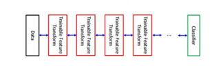
Fig.1. Deep Learning simplified steps
This paper is structured by giving a brief on previous work that was published in finger movement classification and deep learning implementation for the biomedical signal. Very simplified review on the self-organizing map and three bio signal representations (Spectrogram, Wavelet and Wavelet Packet) will be represented where, Discriminate Analysis, Support vector machine, Evolutional Extreme Learning Machine, and Extreme learning machine will be used as an evaluation step. Analysis of Variance (ANOVA) and confidence interval for different classifiers will be calculated. Finally, classifier fusion will be added to improve both training and testing accuracies.
2. Previous Work
In this paper, we will suggest a deep learning model that will be able to learn features by itself without utilising any feature extraction or reduction technique. The proposed model will be skilful in classifying between ten finger movements. Finger movement classification was presented previously in many types of research as in [8] where the researchers proposed a feature projection technique by implementing Fuzzy Neighbourhood Preserving Analysis (FNPA) with QR-decomposition. The primary purpose of Fuzzy Neighbourhood Preserving Analysis (FNPA) is to decrease the distance, to the maximum extent, between samples of the same class and increase it between samples of different classes. The researchers’ purpose was to classify ten finger movements, and they verified average accuracy 91% by using only two channel electrodes. After that, other authors proposed a finger movement classification system. Where, they employed Spectral Regression Discriminant Analysis (SRDA) for dimensionality reduction, Extreme Learning Machine (ELM) for classification and smoothed the results by using majority voting method. They achieved classification accuracy 98% from two electromyography channels only [9]. Then the authors used the same data set collected by using two channel electrodes, which was considered a challenging task, to hire Spectral Regression Discriminate Analysis (SRDA) for dimensionality reduction, kernel-based Extreme Learning Machine (ELM) for classification and smoothed the results by using majority voting method [10]. Moreover, they applied Particle Swarm Optimization (PSO) to optimise the kernel based ELM. Later, other investigators suggested a model classifying between 9 finger movements (classes) by using two electrodes [11]. They implemented seven-time domain features and evaluated the system by applying Artificial Neural Network (ANN) and k- nearest neighbours (KNN) as classifiers. Other investigators suggested using Nonnegative Matrix
Factorization (NMF) technique to select accurate and dependable features. They employed neural networks for classification and calculated the accuracy for both simple and complex flexion where they achieved 95% for simple flexion and 87% for complex one [12]. After that other researchers suggested collecting surface electromyography signal using eight electrodes to classify between nine hand motions. They hired two different neural networks for classification. The first neural network architecture verified 83.43% accuracy while the second one achieved 91.85% [13]. Another experiment was published in [14] where the authors employed time-domain descriptors (TDD) to measure the power spectrum characteristics for electromyography signal which in turn reduced the computationally expensive feature construction traditional techniques. This suggested method improved the error percentage by 8% in comparison with other methods [14]. Another trial was published for recognising finger movements by using microneedle with average accuracy 94.9% [15]. On the other hand, many researchers claimed for implementing a general model that should be able to learn features by itself without employing any feature extraction and reduction techniques which led to deep learning clue. Many published experiments were done in hiring deep learning for biomedical data. As for example but not limited to, in [16] the authors developed a system by using an ensemble of convolutional neural networks to classify medical images. Convolutional neural networks were implemented for learning features by tunning and for classification as well. Other researchers suggested employing convolutional neural networks to learn features and developing low-level features only [17]. The authors in [18] developed a deep learning system to classify between different plaque constituents in Carotid Ultrasound. Later, the texture of lung pattern was analysed by implementing deep learning technique after employing convolutional neural networks [19]. Consequently, we can consider deep learning as a feature learning system where the system will extract the best features suit the application or in another word the system will learn features without employing any feature extraction or feature reduction algorithm. We will propose a deep learning model by engaging self-organising map in learning features from the represented bio signal. The bio signal will be represented using either spectrogram, wavelet or wavelet packet. We will evaluate the behaviour of our suggested model by hiring different classifiers as support vector machine, discriminant analysis, extreme learning machine and evolutionally extreme learning machine. Evolutionally extreme learning machine will lead to higher accuracy results than other implemented classifiers. Analysis of variance and confidence interval for different classifiers will be calculated as well. Finally, and as a development stage, classifier fusion layer will be added to select best local classifier. Accordingly, our proposed model will learn features by itself without hiring any feature extraction or reduction algorithm and verify well-accepted accuracy values. Moreover, implementing analysis of variance and confidence interval is considered as an in-depth step to understand the nature of the relation between our employed classifiers and to know our trustful range of accuracy results.
3. Self-Organizing Map
Self-Organizing Map is a typical artificial neural network which has two main characteristics. The first one is that it follows unsupervised learning technique to generate a lower dimensional copy of input training set. The new dimension of the data is typically two dimensions, and the new training set is called map. While the second characteristic is that it applies error correction by using back propagation technique or gradient descent and at the same time, keeps the properties for the input by using neighbourhood function [7]. Sometimes Self-Organizing Map is called Kohonen map in referring to Teuvo Kohonen who first invented it in 1980 [8]. Self-Organizing Map may represent the nonlinear version of principal component analysis [9]. The new two-dimensional data is considered as the features that will be used for classification steps. SOM is used in unsupervised learning. The network is being trained to generate features from the input data at the output instead of producing classes at the output. The input to the self-organizing map is the represented data either by spectrogram or wavelet or wavelet packet while the output is considered as the features. The classifier uses features produced from the self-organizing map as an input while; its output is the class equivalent to input data. Fig.2 shows the procedures of signal processing by using self-organizing map.
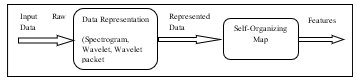
Fig.2. Procedures of SOM signal representation
Fig 3 shows the mapping of a point in the input space to its new point in the output space.
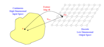
Fig.3. Mapping input space to output space in SOM
In this algorithm, the self-organizing map is being used to reduce the dimension of the data into lower and more useful representation. Consequently, self-organizing map enhances in extracting essential features or good representations of input data. So, the self-organizing map is in the context of feature learning where we have trained data. We will extract some features from training data then, apply the algorithm on the testing set and calculate the classification error.
4. Bio-Signal Processing
4.1. Bio Signal Representation
To improve the performance and to get lower classifier error, we suggest some signal representations can be done on the data before being introduced to the self-organizing map stage. The first data representation is to take the spectrogram of our input data. The spectrogram is to represent the spectrum of frequencies for our signal in a visual manner. Mathematically, Spectrogram can be calculated by taking the square of the magnitude of Short-Time Fourier Transform (STFT) or; it can be named short term Fourier transform. Short time Fourier transform is a Fourier-related transform, where it divides the long-time signal into shorter segments in time. These separated segments should be equal in length and then compute the frequency and phase for each segment separately. So, simply it is Fourier transform but for shorter segments than calculating it for the whole signal at one time[10]. The spectrogram output of the data is being trained by the self-organizing map to extract features then; these extracted features should be used in classification stage. Moreover, wavelet was applied as signal representation Wavelet is considered as small shifted and scaled partitions of the original signal. Fourier transform is representing the signal as a sinusoidal wave with different frequency while wavelet is representing the signal in the form of sharp changes. Wavelet allows us to capture better feature representation for abrupt changes in the signal. However, smooth representation by Fourier is useful in case of the smooth signal. We used Haar wavelet in our software. Fig.4 shows Fourier transform representation and wavelet representation. As a comparative study, we applied wavelet packet for the signal representation. We used six levels for sym10 at sampling frequency 2 kHz.
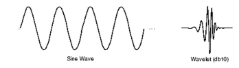
Fig.4. Fourier transforms representation and wavelet representation
4.2 Classifiers
We implemented four classification algorithms, where the first is Extreme Learning Machine (ELM), second is Discriminate Analysis (DA), third is Support Vector Machine (SVM), and the fourth is Self-Adaptive Evolutionary Extreme Learning Machine. We compared the accuracy for six different types of SVM (Linear SVM, Quad SVM, Cubic SVM, Fine Gauss SVM, Medium Gauss SVM and Coarse Gauss SVM) and picked up the most accurate result. Also, we compared Linear Discriminate Analysis (LDA) and Quadrature Discriminate Analysis (QDA) and selected the most accurate result. Fig.5 shows the suggested procedures for our implemented feature learning suggested model
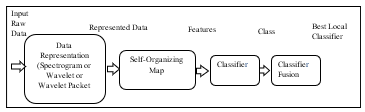
Fig.5. Procedures of Suggested Feature Learning Model
An extreme learning machine is being used in modelling complex systems either linear or nonlinear. The modelling algorithm uses gradient free fast convergence tool [20-23], for N observations {( where . ELM chooses both the input weights and hidden biases in a random manner.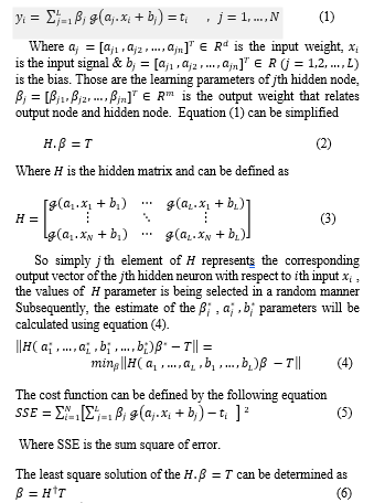
Where is the Moore-Penrose generalized inverse of the hidden layer matrix .
The self-adaptive evolutionary Extreme learning machine introduces the optimisation algorithm by applying differential evolutionary optimisation technique on objective function by picking up a certain number of populations and number of generation until the targeted level of convergence obtained [24-28]. Where, the parameter can be defined as![]()
The procedures of Differential Evolutionary can be defined as following
First, the cover parameter space should be initialized by using the following equation![]()
Where, & are the minimum and maximum boundaries respectively. The values of & are predetermined.
Second, generation of the new mutual vector by calculating difference vectors of randomly picked population vector. These can be calculated by one of four strategies
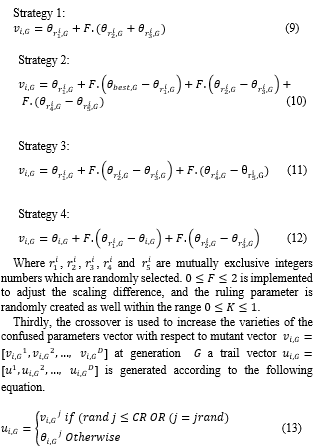
Where is the crossover rate to adjust the friction of the parameter values copied, is evaluation of a uniform random number created in [0, 1] and is randomly selected an integer from [1, D].
Fourthly, Selection is conducted using fitness function for each objective and corresponding trail vector, and the one at a lower value of fitness function is kept as population for the next generation. Then, second and fourth steps are repeated until the objective met or maximum iteration reached.
To overcome the restrictions of mutually selecting trail vector generation strategies and its associated ruling parameters, Self-Adaptive Evolutionary Extreme Learning Machine (SAEELM) is implemented to optimise the ELM output weight matrix using the following procedures
Initialize the hidden layer matrix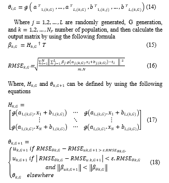
All trail vectors are created the generation are evaluated by implementing equation 16 with small tolerance .
The Analysis of Variance (ANOVA) was calculated for different classifiers. Where, we grouped average testing accuracies for three signal representation techniques (Spectrogram, Wavelet and Wavelet Packet) that result in P value equalled to 0.0613. The P value indicated that there was no practical difference between any of these four classifiers as P value was larger than 0.05 although its value was not that far from 0.05.
Moreover, the Confidence interval for each classifier was calculated with confidence score equals 60%. Generally speaking, confidence interval has two limits one is a higher limit, and the other is the lower one. We are confident in our result by level 60 % as long as testing accuracy, for each classifier, within our interval.
5. Implementation
In this section the data acquisition that we followed will be displayed and explained in more details and results will be discussed.
5.1. Data Acquisition
We used FlexComp Infiniti™ to collect the surface Electromyography signal. MyoScan™ T9503M Sensors were used to obtain two EMG. Those two sensors were put on the subject forearm as shown in Fig.6.
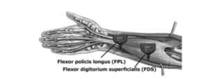
Fig.6. Placement of the electrodes
We have nine subjects where each subject was asked to do one of ten different finger movements for five seconds then take rest for other five seconds. Each movement was reiterated for six times. Then, the subject was asked to perform the same scenario for another finger movement class till finishing the whole ten finger movement classes. The signal was amplified by gain 1000 and sampled at the rate of 2000 sample per second.
The main target is to use collected EMG signal and feature learning technique and classify the finger movement for the subjects into ten classes. Fig.7 shows the targeted ten classes
Three-folded validations for data was used where the training set was 2/3 of the whole data, and the residual 1/3 was assigned for testing set.
The bio signal was filtered to remove any noise that might be superimposed on data. So, the implemented filter was to ensure that our processed signal is free from noise.
The average training and testing accuracy were calculated by simulating the system for each subject separately then summing the training or testing accuracy for all participants and dividing the result by the number of our subjects.
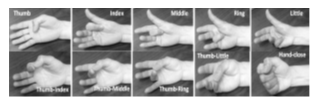
Fig.7. Ten different finger movements
5.2. Results
Table I shows training and testing accuracies for different signal representations and different classifiers
TABLE I. TESTING AND TRAINING ACCURACY
| Signal Representation | Average Training Accuracy | Average Testing Accuracy | Classification Algorithm |
| Spectrogram | 99.41% | 81.54% | Support Vector Machine |
| Spectrogram | 98.26% | 83.29% | Extreme Learning Machine |
| Spectrogram | 96.71% | 91.11% | Evolutionally Extreme Learning Machine |
| Spectrogram | 96.95% | 83.13% | Discriminate Analysis |
| Wavelet | 99.84% | 85.11% | Support Vector Machine |
| Wavelet | 98.03% | 84.91% | Extreme Learning Machine |
| Wavelet | 99.35% | 93.14% | Evolutionally Extreme Learning Machine |
| Wavelet | 98.61% | 86.77% | Discriminate Analysis |
| Wavelet Packet | 98.42% | 90.47% | Support Vector Machine |
| Wavelet Packet | 97.83% | 87.96% | Extreme Learning Machine |
| Wavelet Packet | 99.50% | 94.44% | Evolutionally Extreme Learning Machine |
| Wavelet Packet | 96.30% | 89.98% | Discriminate Analysis |
We went through different experiments by altering self-organizing map configuration until we reached the current configuration where the size of the two-dimensional map was 10×10, the layer topology function employed was ‘hextop’ and the neurone distance function hired was ‘linkdist’. This configuration was to compromise between simulation time and accuracy level. These parameters were optimum regarding the accuracy level and the time consumed in simulation in which, increasing size of our map would recall higher simulation time without a tangible impact on accuracy level. The bio signal was filtered before signal representation stage and neural networks phase to guarantee a substantial barrier against noise level that might be superimposed on our collected bio signal.
The same set of data was introduced to a pattern recognition system, as shown in Fig.8, where we applied the traditional feature extraction and feature reduction techniques. The extracted features were slope sign change, zero crossing, waveform length, skewness, mean absolute value, root mean square and autoregressive. Also, we applied linear discriminant analysis as feature reduction method. The training accuracy was 96.60% and testing accuracy were 88.92%.
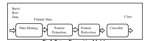
Fig.8. Pattern Recognition Model
It is evident from the results that are shown in Table I that using wavelet packet as a signal representation generated a higher testing accuracy than both wavelet and Spectrogram. Moreover, wavelet had a higher testing accuracy than Spectrogram and had a lower testing accuracy than wavelet packet. Support vector machine showed impressive classification ability for wavelet packet than its ability in spectrogram signal representation. Support vector machine testing accuracy for wavelet packet signal representation was very close to testing accuracy for discriminate analysis classifier but still higher. Moreover, support vector machine showed moderate classification ability for wavelet signal representation and poor classification ability for spectrogram signal representation. On the other side, Extreme learning machine excelled the other classification techniques for spectrogram signal representation. However, testing accuracy for spectrogram signal representation was very close to its value resultant from using Discriminate Analysis classifier. Discriminate analysis showed higher testing accuracy for wavelet signal representation than both extreme learning machine and support vector machine for the same data set and wavelet signal representation while, testing accuracy for wavelet signal representation by using support vector machine was higher than testing accuracy resultant from extreme learning machine for same wavelet signal representation but, close and lower than testing accuracy for discriminate analysis. The testing accuracies, for three signal representations, were moved to another higher level by implementing Evolutionally Extreme Learning Machine as a classifier and this is due to the optimisation algorithm that is being followed by this technique. The only drawback for evolutionally extreme learning machine was its simulation time as it was considered longer than the time consumed during simulation of an extreme learning machine. However, the high accuracy levels gained from evolutionally extreme learning machine was very encouraging to implement it.
We calculated the ANOVA value for four different classifiers. The P value resulted in 0.0613, which is slightly less than 0.05. Although the P value is slightly smaller than 0.05 However, it is yet indicating that there is no sensible difference between those four implemented classifiers
Table II shows the confidence interval for four different performed classifiers
TABLE II. CONFIDENCE INTERVAL for various CLASSIFIERS
Classifier |
Confidence Interval High |
Confidence Interval Low |
Confidence Interval |
Extreme Learning Machine |
86.54% |
84.24% |
2.3% |
Discriminate Analysis |
88.29% |
84.96% |
3.32% |
Support Vector Machine |
87.89% |
83.53% |
4.36% |
Evolutionally Extreme Learning Machine |
93.71% |
92.08% |
1.63% |
Fig.9. Shows the clustered column chart which is representing our confidence interval for our used classifier. The used confidence score is 60%. We are confident in our result by level 60 % as long as testing accuracy, for each classifier, within our interval. It is apparent from these results that evolutionally extreme learning machine has the narrowest range which is 1.63%. Support vector machine has the widest interval, which impacts the gap between higher and lower confidence interval. Moreover, the second widest interval is Discriminate Analysis which results in 3.32% and finally, extreme learning machine generates the second narrowest interval that is 2.3%.
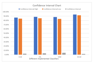
Fig.9. Confidence Interval
Classifier fusion layer was added where; it selected the best local classifier by using dynamic classifier selection algorithm. Both training and testing accuracies were improved as shown in Table III.
TABLE III: CLASSIFIER FUSION TESTING AND TRAINING ACCURACY
| Signal Representation | Average Training Accuracy | Average Testing Accuracy | Classification Algorithm |
| Spectrogram | 98.42% | 93.07% | Classifier Fusion |
| Wavelet | 99.35% | 95.25% | Classifier Fusion |
| Wavelet Packet | 99.73% | 96.60% | Classifier Fusion |
The testing accuracies were improved by adding classifier fusion where wavelet packet testing accuracy exceeded 96% while, wavelet testing accuracy became higher than 95%, and finally, spectrogram became more than 93%. In comparing Table III results with Table I results we can conclude that classifier fusion improved results. Fig.10 shows the number of learned feature for each data representation.
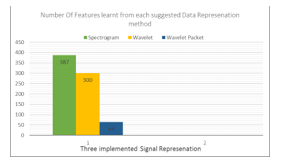
Fig.10. Number of learned features for each data representation
6. Conclusion
The self-organizing map was time-saving and easy feature learning technique, where it reduced dimensions of data without too much loss of the information and observations that should be associated with data. The self-organizing map was considered one of the types of neural networks which use dimension reduction (typically two dimensions) and back propagation for error correction. Although the simulation time was not long, we got a good testing accuracies.
Spectrogram, wavelet and wavelet packet helped in better representing raw data. Support vector machine showed good classification ability in Wavelet Packet while discriminate analysis showed an impressive result in wavelet signal representation and good ability for classification for Spectrogram although Extreme learning machine excelled in Spectrogram testing accuracy than using discriminate analysis.
Evolutionally extreme learning machine was considered a very real improvement for our accuracies percentages. This was due to the optimisation algorithm that existed in the model. As all testing accuracies, for evolutionally extreme learning machine, exceeded 90%. The only drawback for evolutionally extreme learning machine was its simulation time which was relatively longer than that consumed during implementing extreme learning machine. On the other hand, the accuracy values achieved by employing evolutionally extreme learning machine as a classifier was higher than those reached by hiring extreme learning machine in the classification stage.
ANOVA value was 0.0613 as calculated above. The value was not yet to be less than 0.05. However, it was very close to 0.05. This meant that there was no practical difference between classifiers. Despite this, we believed that using evolutionally extreme learning machine pushed ANOVA value to be as close as 0.05.
The confidence interval was calculated by confidence score 60%. And as shown above, the narrowest interval was for an evolutionally extreme learning machine. While the widest range for support vector machine. These intervals gave us an indication of how far we were confident in our resulting testing accuracy. And if the testing accuracy was in our range, so we would be confident in our result by 60%.
Classifier Fusion layer enhanced in increasing testing accuracies for the three used signal representations. Classifier fusion algorithm followed was selecting best local classifier. The only drawback for classifier fusion was increasing simulation time as it became relatively high than before. However, simulation time consumed by the self-organizing map as feature learning was short.
The average simulation time was around 20 seconds which was considered as a short time. However, it was very far from real time hands applications (150m seconds to 300 m seconds). As a future work we are planning to mix all features for three suggested data representation and select top useful features by applying indexing technique then use classifier fusion to combine between reaching real simulation time in real hands applications (150m seconds to 300 m seconds) and verifying high testing accuracies rate. Also, as a future work, we are planning to introduce raw data to our model without any signal representation to save simulation time and build a practical system.
- M. F. I. I. A. A. Al-Jumaily, “PCA indexing based feature learning and feature selection,” presented at the 2016 8th Cairo International Biomedical Engineering Conference (CIBEC), Cairo, Egypt, 2017.
- R. Dechter, “Learning While Searching in Constraint-Satisfaction-Problems,” presented at the Proceedings of the 5th National Conference on Artificial Intelligence, Philadelphia, 1986.
- L. Y. Deng, D, “Deep Learning: Methods and Applications,” Foundations and Trends in Signal Processing, vol. 7, pp. 3-4, 2014.
- Y. Bengio, “Learning Deep Architectures for AI,” Foundations and Trends in Machine Learning, vol. 2, no. 1, pp. 1-127, 2009.
- Y. C. Bengio, A.; Vincent, P., “Representation Learning: A Review and New Perspectives,” IEEE Transactions on Pattern Analysis and Machine Intelligence, vol. 35, no. 8, pp. 1798–1828, 2013.
- J. Schmidhuber., “Learning complex, extended sequences using the principle of history compression,” Neural Computation, vol. 4, pp. 234–242, 1992.
- G. E. Hinton, “Deep belief networks,” Scholarpedia, vol. 4, no. 5, p. 5947, 2009.
- S. K. Rami N. Khushaba, Dikai Liu, Gamini Dissanayake, “Electromyogram (EMG) Based Fingers Movement Recognition Using Neighborhood Preserving Analysis with QR-Decomposition,” presented at the 2011 Seventh International Conference on Intelligent Sensors, Sensor Networks and Information Processing, Adelaide, SA, Australia, 2011.
- R. N. K. a. A. A.-J. Khairul Anam, “Two-Channel Surface Electromyography for Individual and Combined Finger Movements,” presented at the 35th Annual International Conference of the IEEE EMBS, Osaka, Japan, 2013.
- K. A. a. A. Al-Jumaily, “Swarm-based Extreme Learning Machine for Finger Movement Recognition,” presented at the 2014 Middle East Conference on Biomedical Engineering (MECBME), Doha, Qatar, 2014.
- M. H. P. C. B. V. Rao, “EMG signal based finger movement recognition for prosthetic hand control,” presented at the Communication, Control and Intelligent Systems (CCIS), 2015, Mathura, India, 2015.
- G. R. N. a. H. T. Nguyen, “Nonnegative Matrix Factorization for the Identification of EMG Finger Movements: Evaluation Using Matrix Analysis,” IEEE JOURNAL OF BIOMEDICAL AND HEALTH INFORMATICS, vol. 19, no. 2, pp. 478-485, 2015.
- S. H. Rocio Alba-Flores, and A. Shawn Mirzakani, “Performance Analysis of Two ANN Based Classifiers for EMG Signals to Identify Hand Motions,” presented at the SoutheastCon, 2016, Norfolk, VA, USA, 2016.
- A. H. A.-T. Rami N. Khushaba, Ahmed Al-Ani, and Adel Al-Jumaily, “A Framework of Temporal-Spatial Descriptors based Feature Extraction for Improved Myoelectric Pattern Recognition,” IEEE Transactions on Neural Systems and Rehabilitation Engineering, vol. PP, no. 99, 2016.
- D. S. K. Minjae Kim, and Wan Kyun Chung, “Microneedle-Based High-Density Surface EMG Interface with High Selectivity for Finger Movement Recognition,” presented at the 2016 IEEE International Conference on Robotics and Automation (ICRA), Stockholm, Sweden, 2016.
- J. K. shnil Kumar, David Lyndon, Michael Fulham, and Dagan Feng, “An Ensemble of Fine-Tuned Convolutional Neural Networks for Medical Image Classification,” IEEE JOURNAL OF BIOMEDICAL AND HEALTH INFORMATICS, vol. 21, no. 1, pp. 31-40, 2016.
- Y. Z. Ruikai Zhang, Tony Wing Chung Mak, Ruoxi Yu, Sunny H. Wong, James Y. W. Lau, and Carmen C. Y. Poon, “Automatic Detection and Classification of Colorectal Polyps by Transferring Low-Level CNN Features From Nonmedical Domain,” IEEE JOURNAL OF BIOMEDICAL AND HEALTH INFORMATICS, vol. 21, no. 1, pp. 41 – 47 2016.
- A. G. Karim Lekadir, An` angels Betriu, Maria del Mar Vila, Laura Igual, Daniel L. Rubin, Elvira Fernandez, Petia Radeva, and Sandy Napel, “A Convolutional Neural Network for Automatic Characterization of Plaque Composition in Carotid Ultrasound,” IEEE JOURNAL OF BIOMEDICAL AND HEALTH INFORMATICS, vol. 21, no. 1, pp. 48 – 55, 2016.
- M. A. Stergios Christodoulidis, Lukas Ebner, Andreas Christe, and Stavroula Mougiakakou, “Multisource Transfer Learning With Convolutional Neural Networks for Lung Pattern Analysis,” IEEE JOURNAL OF BIOMEDICAL AND HEALTH INFORMATICS, vol. 21, no. 1, pp. 76 – 84 2016.
- Z. Q.-Y. Huang G-B, Siew C-K, “Extreme learning machine: a new learning scheme of feedforward neural networks,” In Proceedings of the international joint conference on neural networks, Budapest, Hungary, pp. 985–990, 2004.
- Z. Q.-Y. Huang G-B, Siew C-K, “Extreme learning machine: theory and applications.,” Neurocomputing, vol. 70, no. 1-3, pp. 489–501, 2006.
- J. Tang, C. Deng, and G. B. Huang, “Extreme Learning Machine for Multilayer Perceptron,” IEEE Transactions on Neural Networks and Learning Systems, vol. 27, no. 4, pp. 809-821, 2016.
- Y. Miche, A. Sorjamaa, P. Bas, O. Simula, C. Jutten, and A. Lendasse, “OP-ELM: Optimally Pruned Extreme Learning Machine,” IEEE Transactions on Neural Networks, vol. 21, no. 1, pp. 158-162, 2010.
- J. Cao, Z. Lin, and G.-B. Huang, “Self-Adaptive Evolutionary Extreme Learning Machine,” Springer Science+Business Media, LLC. 2012, 18 July 2012 2012.
- L. D. S. Pacifico and T. B. Ludermir, “Evolutionary extreme learning machine based on particle swarm optimisation and clustering strategies,” in Neural Networks (IJCNN), The 2013 International Joint Conference on, 2013, pp. 1-6.
- N. Zhang, Y. Qu, and A. Deng, “Evolutionary Extreme Learning Machine Based Weighted Nearest-Neighbor Equality Classification,” in 2015 7th International Conference on Intelligent Human-Machine Systems and Cybernetics, 2015, vol. 2, pp. 274-279.
- K. F. Man, K. S. Tang, and S. Kwong, “Genetic algorithms: concepts and applications [in engineering design],” IEEE Transactions on Industrial Electronics, vol. 43, no. 5, pp. 519-534, 1996.
- S. Jie, Y. Yongping, W. Peng, Y. Liu, and H. Shuang, “Genetic algorithm-piecewise support vector machine model for short-term wind power prediction,” in Intelligent Control and Automation (WCICA), 2010 8th World Congress on, 2010, pp. 2254-2258.