1            Introduction

In recent years, the control of chaotic systems has increasingly interested researchers. The first chaos control method has been proposed by Ott et al. [1], nowadays known as the OGY (Ott-Grebogi-Yorke) method. This is a discrete technique that considers small perturbations applied in one system parameter when the trajectory approaches the vicinity of the desired orbit when crossing a specific surface. Since then, numerous control techniques have been proposed for controlling chaos in different chaotic systems such as backstepping [2–4], adaptive control algorithms [5–7] and sliding-mode control [8–10].

The sliding mode control (SMC) has undergone extensive and detailed studies in the last three decades. It is noted that SMC is a powerful robust control strategy treating the model uncertainties and external disturbances. The design and the implementation of discrete time sliding mode control have later been considered, and still in progress because a large classes of continuous systems are controlled by digital signal processors and microprocessors. Indeed, discrete sliding mode control is well studied in the literature [11–14]. The aim of this work is to give a further contribution in this field. The main objective is to design a discrete time sliding mode control strategy and enhanced by a stable adaptive fuzzy inference system to cope with modeling inaccuracies and external disturbances that can arise. Many researches on introducing the concept of fuzzy logic and especially fuzzy approximators into sliding mode control have been developed in the past years [15–18]. Historically, fuzzy logic systems have been proposed in an attempt to control nonlinear systems whose parameters are inaccuracy, and presenting neglected dynamics as well as time varying systems [19]. Since then, fuzzy logic control becomes an active research area and it has been implemented in several industrial applications. Accordingly, fuzzy logic with discrete sliding mode control are proposed to improve system control performances. Thus, the overall control system drives the tracking error to zero even in the presence of external disturbances. This paper is organized as follows: Section 2 and 3 deal with discrete sliding mode and fuzzy system respectively. Moreover, the detailed design procedure of fuzzy sliding mode controller is explained in section 4. Numerical simulations are carried out in section 5 for illustration and verification of the proposed controller. Finally, some concluding remarks are given in section 6.

2          Discrete-time sliding mode controller

Consider the following nonlinear discrete time system

                   x1(k +1) = x2(k)                      x2(k +1) = x3(k)                                   …                       xn−1(k +1) = xn(k)      x (k +1) = f (x(k))+u(k)+d(k)

(1)

_n

where x(k) = [x₁(k),x₂(k),…,x_n(k)]^T is the state vector and u(k) is the input signal.

f (x(k)) is unknown but it is a bounded function and d(k) is a bounded external disturbance such that |d(k)| < D.

When u(k) = 0, system (1) behaves chaotically. Therefore, the aim of this work is to apply a discrete-time sliding mode controller u(k) in order to track a desired trajectory.

Let x_d(k) = [x_d1(k),x_d2(k),…,x_dn(k)]^T the well known desired trajectory. Then, the tracking error can be expressed as

                                 e(k) = x(k) − x_d(k)                                     (2)

where e(k) = [e₁(k),e₂(k),…,e_n(k)]^T .

The sliding surface can be defined as

     s(k)     =             c₁e₁(k)+c₂e₂(k)+…+c_n−1e_n−1(k)+e_n(k)

                =      Ce(k) = 0                                                            (3)

where C = [c₁,c₂,…,c_n−₁,1] can be selected as h(z) = zⁿ⁻¹+c_n−₁zⁿ⁻²+…+c₂z+c₁ is stable. The sliding mode controller is designed by adopting the reaching law defined by [12]

∆s(k +1) = s(k +1) − s(k) = −Qs(k) − Ksign(s(k)) where 0 < Q < 1 and K > 0. If f (x(k)) is supposed known and d(k) = 0 then	(4)
n−1 X s(k +1) =           ciei(k +1)+f (x(k))+u(k) − xdn(k +1) i=1 therefore ∆s(k +1) can be expressed as n−1 X ∆s(k +1)      =                ciei(k +1)+f (x(k))+u(k) i=1	(5)
n−1 X −      xdn(k +1) −          ciei(k) − en(k)	(6)

i=1

The equivalent control u_eq(k) can be derived by using ∆s(k +1) = 0 such that

n−1

X

       u_eq(k)     =     −            c_ie_i(k +1) − f (x(k))+x_dn(k +1)

i=1

n−1

X

                       +              c_ie_i(k)+e_n(k)                                         (7)

i=1

Since d(k) , 0 then a switching type control must be added such that u(k)              =              u_eq(k)+u_s(k)

n−1

X

                     =     −            c_ie_i(k +1) − f (x(k))+x_dn(k +1)

i=1

n−1

X

                     +                c_ie_i(k)+e_n(k)+u_s(k)                              (8)

i=1

where u_s(k) is defined by

                         u_s(k) = −Qs(k) − Ksign(s(k))                            (9)

where the switching gain K will be determined afterwards .

Furthermore, if f (x(k)) is unknown then a fuzzy system fˆ(x(k)) will be used to approximate f (x(k)) in order to obtain the sliding mode control law. Moreover, an adaptive adjusting law will be designed.

3          Fuzzy system

The knowledge base for the fuzzy logic system comprises a collection of fuzzy IF-THEN rules of the form:

            (j)                                                    j                                                       j

          R₁ :         If             (x₁(k) is A₁)…and (x_n(k) is A_n)

                      then        h(y(x(k)) = b^j)ⁱ                                   (10)

pour j = 1,…,H. H is the rule number of the fuzzy logic system.

x_i(k), i = 1,…,n and y(x(k)) denote the linguistic variables associated with the inputs and the output of the fuzzy logic system.

By the use of the singleton fuzzification strategy, product inference and center-average defuzzification, the output of the fuzzy system is expressed as:

PH           yj(x(k))Qni=1µAji (xi(k)) j=1

            y(x(k))      ⁼   _{P       Q}                       (11)

                                              Hr=1          np=1µ_Arp(x_p(k))

where µ j is the membership function of the linguis-

A_i

j tic variable A_i .

By introducing the concept of fuzzy basis function vector ξ(x(k)) , (11) can be rewritten as:

y(x(k)) = θT ξ(x(k)) where	(12)
 y1(x(k))                                ξ1(x(k))      θ =  :  , ξ(x(k)) =  :              H(x(k))                 ξH(x(k))  y and	(13)
Qn          µ j (xi(k)) j(x) =               i=1 Ai                                  ξ	(14)

PHr=1 Qnp=1µArp(xp(k))

ξ^j(x(k)) which are called fuzzy basis functions (FBF’s). It has been proved that these FBF’s are universal approximators [20].

4          Fuzzy Sliding mode control

In order to derive the sliding mode control, the fuzzy system fˆ(x(k)/θ_f ) is used to approximate f (x(k)) [21].

The fuzzy logic system fˆ(x(k)/θ_f ) is expressed by:

www.astesj.com                                                                                                                                                                                 396

                            f^ˆ(x(k)/θ_f ) = θ_f^T ξ_f (x(k))                             (15)

where ξ_f (x(k)) is the vector of fuzzy basis supposed to be fixed, while parameters θ_f are variables which will be designed by adaptive laws.

Let θ_f^∗ the optimal parameter vectors of the fuzzy logic system. Minimum approximation error can be defined as follows:

                   w_f (k) = f (x(k)) − f^ˆ(x(k)/θ_f^∗ )+d(k)                      (16)

Then, we can select the control law as: u(k)  =              u_eq(k)+u_s(k)

n−1

                  =            ^−Xc_ie_i(k +1) − f^ˆ(x(k)/θ_f )+x_dn(k +1)

i=1

n−1

X

                  +                      c_ie_i(k)+e_n(k) − Qs(k) − Ksign(s(k))(17)

i=1

where 0 < Q < 1 and K will be determined afterwards. Therefore, ∆s(k +1) can be rewritten as

∆s(k +1)       =            f (x(k)) − f^ˆ(x(k)/θ_f ) − Qs(k) − Ksign(s(k))

                      −       Qs(k) − Ksign(s(k))

= Φ_f^T (k)ξ_f (x(k))+w_f (k)

                      −       Qs(k) − Ksign(s(k))                                    (18)

where Φ_f (k) represent the fuzzy parameter errors such that:

                               )                                  (19)

Theorem 1 The following adaptive law for adjusting the parameter vector θ_f

                            ∆θ_f (k) = −αξ_f (x(k))s(k)                                (20)

asymptotically stabilizes system (1) controlled by (17), where α is a positive constant which determines the rate of adaptation.

Proof: The Lyapunov function candidate is chosen as

V (k) = 21s²(k)+ ¹ Φ_f^T (k − 1)Φ_f (k − 1)          (21) 2α

Then, ∆V (k) can be obtained as

∆V (k +1)          =      V (k +1) − V (k)

                          =     12s²(k +1) − s²(k)+ 2¹αΦ_f^T (k)Φf (k)

                                   1      f^T (k − 1)Φ_f (k − 1)                         (22)

−Φ

2α

Let

∆θ˜_k = 2¹αΦ_f^T (k)Φf (k) − 2¹αΦ_f^T (k − 1)Φf (k − 1)          (23) then

1 ²(k +1) −s²(k)+∆θ˜_k

              ∆V (k +1) =      s

2

     =          (∆s(k +1)+s(k))² − s²(k)+∆θ˜_k

     =          ∆s(k +1)² +s(k)∆s(k +1)+∆θ˜_k

     =       ∆s(k +1)² +∆θ˜_k

     +                 s(k)^hΦ_f^T (k)ξ_f (x(k))+w_f (k) − Qs(k) − Ksign(s(k))ⁱ

     =           ∆s(k +1)² +s(k)Φ_f^T (k)ξ_f (x(k))+s(k)w_f (k)

     −        Qs²(k) − Ks(k)sign(s(k))+∆θ˜_k                                                 (24)

Moroever, ∆θ˜_k can be transformed as

∆θ˜_k = 2¹αΦ_f^T (k)Φ_f (k) − 2¹αΦ_f^T (k − 1)Φ_f (k − 1)

                 1       ^T (k)Φf (k)

        =      2αΦ_f

                 1                                    ^T (Φ_f (k) − ∆Φ_f (k))

−     (Φ_f (k) − ∆Φ_f (k)) 2α

              α1          ^T (k)∆Φf (k) −∆Φ_f^T (k)∆Φf (k)                      (25)

= Φ_f

Substituting (25) into (24), we obtain

∆V (k +1) = ∆s(k +1)² +s(k)Φ_f^T (k)ξ_f (x(k))

     +        s(k)w_F(k) − Qs²(k) − Ks(k)sign(s(k))

           α1          ^T (k)∆Φ_f (k) −∆Φ_f^T (k)∆Φ_f (k)

+ Φ_f

= ∆s(k +1)² +s(k)w_f (k) − Qs²(k) − Ks(k)sign(s(k)) + Φ_f^T (k)(s(k)ξ_f (x(k))+ ∆Φ_f (k))

     −      ∆Φ_f^T (k)∆Φ_f (k)                                                      (26)

By applying the adaptive law (20), equation (26) can be rewritten as

∆V (k +1) = ∆s(k +1)² +s(k)w_F(k) − Qs²(k)

                  −Ks(k)sign(s(k)) − ∆Φ_f^T (k)∆Φ_f (k)                 (27)

According to (18), we have

||

                                      +    |Qs(k)| + |Ksign(s(k))|             (28)

Furthermore,        it’s           obvious  that         ξ_f (x(k))   remains bounded such that

                              kξ_f (x(k))k ≤ ψ_ξ ∀k ≥ 0                                (29)

where ψ_ξ is a positive constant. According to (20) and (29) and from k > N₀, we have

|∆θf (k)| ≤ ψθ|s(k)| where ψθ is positive constant. Consequently, we can deduce that	(30)
|Φf (k)| ≤ ψΦ|s(k)|	(31)

It is obvious that the term |w_f (k)| ≤ ψ_w where ψ_w is a positive constant. If we define u_sgn = −Ksign(s(k)) then

|∆s(k +1)|	≤	ψξψΦ|s(k)| +ψw +Q|s(k)| + |usgn|
	≤	(ψξψΦ +Q)|s(k)| +ψw + |usgn|
	≤	β|s(k)| +(ψ     +K)                             (32)

_w

where β = (ψ_ξψ_Φ + Q). By taking square from both sides of (32), we can get

                 |∆s(k +1)^|2        ≤       β²|s(k)^|2 +(ψ_w +K)²

                                           +      2β|s(k)|(ψ_w +K)                   (33)

Then,

|

Thus, we can obtain

|s(k)|² +β|s(k)|(ψ_w +K)

          −    Q|s(k)|2 +K|s(k)| +ψw|s(k)| − ψw|s(k)|

|

(35)

If we choose

                                                  1 ²                                                                 (36)

                                        Q >     β

2

and

r

K          =         − (β +1)+                      [(β +1)² +2(Q −β²)] |s(k)|

− then	ψw			(37)
	(ψw +K)2	+	(β +1)|s(k)|(ψw +K)

                                            +      (β² − Q)|s(k)|² = 0            (38)

Therefore, (27) can be expressed as

|

1

                                          −             ∆Φ (k)∆Φf (k)                (39)

It’s clear that s(k)w_f (k)−ψ_w|s(k)| ≤ 0 since |w_f (k)| ≤ ψ_w, furthermore    0, then

                                     ∆V (k +1) ≤ 0                                      (40)

By using the Barbalat’s lemma [23], we can readily prove that s(k) → 0 as k → +∞ thus lim e(k) = 0.

k→+∞

5          Simulation results

To illustrate the above design approach, a 3D Henon chaotic model is considered.

The model for the discrete-time 3D Henon map is given as [22]

  1(k +1) x    (k +1) x2   x3(k +1)      

= x2(k) = x3(k) = −0.2x1(k) − 0.3x2(k) − 1.65x3(k) − x32(k) +u(k)

(41)

The non controlled (u(k) = 0) Henon map has a chaotic strange attractor. The result of computation is shown in figure 1 where [x₁(0),x₂(0),x₃(0)]^T = [0.1,0,0.1]^T .

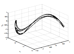Figure 1: Henon map attractor.´

In order to control this autonomous chaotic system, controller u(k), given by (8), is applied at k = 60 to reach the desired trajectory x_d(k) = [0,0,0]^T .

For the estimation of f (x(k)), we consider five fuzzy levels, i.e. NB, NS, EZ, PS and PB on x₁, x₂ and x₃. We use fuzzy logic systems with center-average defuzzifier, product inference, singleton fuzzifier and Gaussian membership functions to approximate f (x(k)). Slopes c_i are chosen as c₁ = 0.1 and c₂ = 0.9.

In figure 2, we represent the evolution of system states which converge rapidly to the desired values. Figure 3 represent the sliding surface and the control signal whose amplitude is always within an acceptable range compared to the system states.

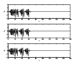Figure 2: Evolution of system states

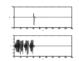Figure 3: Representation of the sliding surface and the fuzzy sliding mode controller.

In order to illustrate the robustness of our design, a white gaussian noise with variance equal to 0.01 has been considered as an external disturbance. The control objective has been achieved as is illustrated in figures 4 and 5. Thus, the robustness of the discrete fuzzy sliding mode controller is proved.

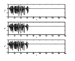Figure 4: Evolution of system states in presence of a white gaussian noise.

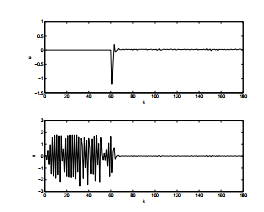Figure 5: Representation of the sliding surface and the fuzzy sliding mode controller.

6          Conclusion

In this paper, an adaptive discrete-time fuzzy sliding mode controller is proposed. This controller, inherits the advantages of both sliding mode control and fuzzy systems. It has been proposed for stable control of a class of chaotic systems. The sliding mode control is proposed as a robust method to control nonlinear and uncertain systems. Consequence parameters of fuzzy control rules have been adjusted on-line in order to guarantee the reaching condition. Simulation results of a 3D Henon chaotic model show the applicability and the effectiveness of the proposed approach.

Conflict of Interest The authors declare no conflict of interest.

1. E. Ott, C. Grebogi, J. A. Yorke, “Controlling chaos”, Physical Review Letters, 64, 1196–1199, 1990.
2. X. Tan , J. Zhang, Y. Yang, “Synchronizing chaotic systems using backstepping design”, Chaos, Solitons and Fractals, 16, 37–45, 2003.
3. J. H. Park, “Synchronization of Genesio chaotic system via backstepping approach”, Chaos, Solitons and Fractals, 27(5), 1369–1375, 2006.
4. H. Adelipoor, O.A. Babaei, “Stability and Tracking in the New Chaotic System Using Backstepping Method”, J. Basic. Appl. Sci. Res., 3, 446–452, 2013.
5. H.Zhang, H. Quin, G. Chen, “Adaptive control of chaotic systems with uncertainties”, Int. J. Bifurcation and Chaos, 8(10), 2041–2046, 1998.
6. M. Feki, “Model-independent adaptive control of chua’s system with cubic nonlinearity”, Int. J. Bifurcation and Chaos, 14(12), 4249–4263, 2004.
7. M. P. Aghababa, B. Hashtarkhani, “Synchronization of Unknown Uncertain Chaotic Systems Via Adaptive Control Method”, Journal of Computational and Nonlinear Dynamics, 10(5), 051004, 2015.
8. H.T. Yau, C.K. Chen, C. Li Chen , “Sliding mode control of chaotic systems with uncertainties”, Int. J. Bifurcation and Chaos, 10(5), 1139–1147, 2000.
9. J. J. Yan, Y. S. Yang, T. Y. Chiang, C. Y. Chen, “Robust synchronization of unified chaotic systems via sliding mode control”, Chaos, Solitons and Fractals, 34(3), 947–954, 2007.
10. M. Feki, “Sliding mode control and synchronization of chaotic systems with parametric uncertainties”, Chaos Solitons and Fractals, 41(3), 1390–1400, 2009.
11. K. Furuta, “Sliding mode control of a discrete systems”, Systems and Control Letters, 14(2), 145–152, 1990.
12. W. Gao, Y. Wang, A. Homaifa, “Discrete-time variable structure control systems”, IEEE Trans. Ind. Electronics, 42(2), 117–122, 1995.
13. H. Sira-Ramirez, “Non-linear discrete variable structure systems in quasi-sliding mode”, International Journal of Control, 54(5), 1171–1187, 1991.
14. S.Z. Sarpturk, Y. Istefanopulos, O. Kaynak, “On the stability of discrete-time sliding mode systems”, IEEE Transaction Automatic Control, AC-32(10), 930–932, 1987.
15. J.Y. Chen, “Rule regulation of fuzzy sliding mode controller design: direct adaptive approach”, Fuzzy sets and systems, 120, 159–168, 2001.
16. O. Kaynak, “Fuzzy adaptive sliding mode control of a direct drive robot, Robotics and Autonomous Systems”, 19, 215–227, 1996.
17. H. Medhaffar, T. Damak, N. Derbel, “A decoupled fuzzy indirect adaptive sliding mode controller with application to robot manipulators”, IJMIC, 1(1), 23–29, 2006.
18. H. Medhaffar, T. Damak, N. Derbel, “Direct adaptive fuzzy moving sliding mode controller design for robotic manipulators”, IJCIA, 5(1), 1–20, 2005.
19. L.A. Zadeh, “Outline of a new approach to the analysis of complex systems and decision processes”, IEEE Trans. Systems, Man. cybernetics, 3(1), 28–44, 1973.
20. L.X. Wang, Adaptive fuzzy systems and control, Englewood Cliffs, NJ: Prentice-Hall, 1994.
21. B. Yoo, W. Ham, “Adaptive fuzzy sliding mode control of nonlinear systems”, IEEE Trans. Fuzzy systems, 6(2), 315–321, 1998.
22. S. V. Gonchenko, I. I. Ovsyannikov, C. Simo, D. Turaev, “Three Dimensional Henon-like Maps” and Wild Lorenz-like Attractors”, International Journal of Bifurcation and Chaos, 15 (11), 3493–3508, 2005.
23. J. J. E. Slotine, W. Li, Applied Nonlinear Control, Englwood Cliffs, NJ:Prentice Hall, 1991.

(Click to view)

(Click to view)