A Computationally Intelligent Approach to the Detection of Wormhole Attacks in Wireless Sensor Networks
A Computationally Intelligent Approach to the Detection of Wormhole Attacks in Wireless Sensor Networks
Volume 2, Issue 3, Page No 302-320, 2017
Author’s Name: Mohammad Nurul Afsar Shaon, Ken Ferensa)
View Affiliations
University of Manitoba, Electrical and Computer Engineering, R3T2N2, Canada
a)Author to whom correspondence should be addressed. E-mail: Ken.Ferens@umanitoba.ca
Adv. Sci. Technol. Eng. Syst. J. 2(3), 302-320 (2017); ![]() DOI: 10.25046/aj020340
DOI: 10.25046/aj020340
Keywords: Artificial Intelligence, Wormhole attack, Non-uniform Sensor distribution, In-band wormhole attack, Out of band wormhole attack, Neighborhood counts, Average residual energy pattern

Export Citations
A wormhole attack is one of the most critical and challenging security threats for wireless sensor networks because of its nature and ability to perform concealed malicious activities. This paper proposes an innovative wormhole detection scheme to detect wormhole attacks using computational intelligence and an artificial neural network (ANN). Most wormhole detection schemes reported in the literature assume the sensors are uniformly distributed in a network, and, furthermore, they use statistical and topological information and special hardware for their detection. However, these schemes may perform poorly in non-uniformly distributed networks, and, moreover, they may fail to defend against “out of band” and “in band” wormhole attacks. The aim of the proposed research is to develop a detection scheme that is able to detect all kinds of wormhole attacks in both uniformly and non-uniformly distributed sensor networks. Furthermore, the proposed research does not require any special hardware and causes no significant network overhead throughout the network. Most importantly, the probable location of the malicious nodes can be identified by the proposed ANN based detection scheme. We evaluate the efficacy of the proposed detection scheme in terms of detection accuracy, false positive rate, and false negative rate. The performance of the proposed algorithm is also compared with other machine learning techniques (i.e. SVM and regularized nonlinear logistic regression (LR) based detection models). The simulation results show that proposed ANN based algorithm outperforms the SVM or LR based detection schemes in terms of detection accuracy, false positive rate, and false negative rates.
Received: 06 March 2017, Accepted: 26 April 2017, Published Online: 14 May 2017
1. Introduction
Wireless sensor networks (WSNs) consist of self-directed devices (i.e., sensor nodes), which are used in a collective manner to monitor environmental or physical phenomena in a remote and/or hostile environment. Spatially distributed autonomous sensor nodes are capable of communicating amongst themselves in order to transfer sensed data to a base station. The WSN is a type of ad-hoc network that has gained popularity for its versatile application in military and civil domains such as battlefield monitoring, tracking objects, healthcare, and home automation[1].
In WSN, a larger number of sensor nodes perform an assigned task in a hostile environment without any human intervention. Since sensor nodes use a known in-band radio channel for communication and are usually deployed in a hostile or remote environment, therefore, WSNs are prone to various security threats like a Sinkhole attack, Sybil attack, and wormhole attack. WSN has several vulnerabilities that an attacker can exploit to obtain access to the network. Implementing security measures like data encryption is not practical solution for the most WSNs. However, research on security measures has made certain progress in secure localization algorithm, lite weight routing protocols, and secure data aggregation scheme. However, those security mechanisms don’t provide any protection against any attack from a legitimate node. If an attacker gains control over a few legitimate nodes, full access would be gained to the data traveling through these compromised nodes. The attacker may achieve the capability to modify the contents of the control packets later by extracting the cryptographic contents from the captured data packets.
Wormhole attack is recognized as one of the most detrimental security threats for any routing protocol of WSNs [2-3]. The wormhole attack can be easily launched by taking over at least two legitimate nodes from the two distant parts of the network or deploying two nodes with superior capabilities (e.g. directional antenna, larger radio range) in two distant places of the sensor field. Wormhole nodes are connected through a virtual tunnel which can be implemented in numerous ways (e.g. high-quality channel, packet encapsulation or packet relay and high powered transmission) [4]. This direct low latency tunnel is known as a wormhole link [5]. A wormhole link creates an illusion in the network that these two colluding nodes are located within their communication range, but, in fact, their physical locations are very far apart.
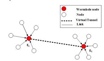
Fig. 1 Depiction of the structure of a wormhole attack.
By creating this unauthorized link, wormhole nodes gain the ability to circulate false route information into the network that they are few hops away from the base stations. This illusion drives other sensor nodes to transmit data packets to the base station through the wormhole nodes. Wormhole attack disrupts the existing network data flow in order to monitor and capture the data packets passing through it. As shown in Fig. 1, the and wormhole nodes, connected by a wormhole link, capture the data packets from one terminal of the virtual tunnel and retransmit them to another terminal of that link.
Subsequently, this wormhole attack becomes so severe that it might destroy the network or hamper the usual operation of the network by the selective dropping of packets, manipulation of traffic, or modify data packets without revealing their identities.
Therefore, detection of wormhole nodes is an essential task for ensuring the security of wireless sensor networks. It is a very simple task to implement wormhole attack, but a very difficult task to detect an infected network since wormhole nodes retransmit valid packets into the network. Most of the existing countermeasures use the distance bounding technique, direction, and location abnormality among claimed neighbor nodes as detection attributes to fight against wormhole attack. To gain a certain level of accuracy, some existing schemes uses complex and highly advanced devices such as directional antenna[6], GPS[7], or ultrasound for distance measurement [8]. However, those special devices are very costly for practical deployment. A few statistical wormhole detection schemes based on hop count [9], node connectivity [5], or neighborhood count [10-12] are proposed that do not need any special hardware. However, they usually include a hardware supported scheme as a secondary approach. Furthermore, centralized statistical wormhole detection [10] may cause significant network and communication overhead in contrast to a distributed statistical approach [11]. In the network connectivity based wormhole attack detection schemes [5,13-14], the positions of neighboring nodes are estimated from the received signal strength (RSSI ) by each node, which sends this information to the base station. By doing this, the network layout is determined by the base station and compared with the given network layout. This approach also causes a significant amount of control packets flow to the base station. Moreover, it is prone to distance estimation errors. Furthermore, neighborhood-based wormhole detection schemes [10,12] may not detect wormhole attack if the wormhole nodes are located in a sparsely populated area and caused the significant flow of packets to the base station. In addition, their performance in non-uniform sensor distribution is in question.
In recent years, network anomaly detection schemes have been increasingly using artificial intelligence to improve detection accuracy. An artificial neural network (ANN) is a very simplified information processing model that aims to grossly imitate the human brain function. An ANN consists of interconnected processing units and works in a parallel fashion to find a solution to a particular non-linear problem. The adaptive and self-learning ability of an ANN help to increase the competence of an anomaly detection model [15]. Moreover, ANNs have been widely deployed to deal with pattern recognition and classification problems [16].
In this paper, we introduce a novel detection scheme based on an ANN using ‘neighborhood count’ and ‘average residual energy pattern of neighbors (AREPN)’ as detection attributes. The proposed detection scheme is able to detect wormhole attacks in both uniform and non-uniform sensor distributions and does not need any special hardware. Here, we have introduced a mobile node, called as detector node ( ) that visits randomly chosen locations within the region of interest and collects two featured data samples, along with coordinate for each site visited. When the detector node moves into a wormhole infected zone, this paper theorizes that the collected number of neighbors increases abnormally (uniform network scenario) or slightly abnormally (non-uniform network scenario), compared to a non-infected zone, in which the counts change normally. This paper also introduces a new detection attribute, named AREPN that significantly decreases at the wormhole infected zone compare to non-infected zone. captures these features as evidence of the presence or absence of a wormhole attack. The gathered dataset is used for training in the proposed ANN based detection scheme. After the training phase, the test data samples are fed into the ANN, and the scheme decides if there is any wormhole attack in the network or not.
We have studied in detail and compared the performance of the proposed algorithm with SVM and LR based detection schemes through simulations. Our simulation results confirm that an ANN based wormhole detector can detect wormhole attacks with higher precision and accuracy as compared to the non-linear logistic classification algorithm.
The rest of this paper is arranged as follows: Section 3 presents a detail of wormhole attack and its classification. We discuss literature review, ANN, SVM and LR in Section 3, 4, 5, and 6, respectively. The proposed ANN-based detections scheme described in detail in Section 7. The evaluation results are discussed in Section 8. Section 9 concludes the paper and provide a scope of future work.
2. Wormhole attacks
A wormhole can be a severe attack against any packet routing protocol, especially in ad-hoc and wireless sensor networks. It is very difficult to detect and to take preventive measures against wormhole attack since the malicious nodes behave as legitimate nodes and initially do not perform any illegal activity in the network[2]. The word ‘wormhole’ means the creation of any shortcut path between two far apart points in the space-time [17]. Thus, the concept of ‘wormhole’ is used as a tool to launch this attack aiming to spoil the existing routing protocol.
The wormhole attack starts by compromising at least two nodes from the sensor network by hacking or, deploying two nodes with superior capabilities (e.g. directional antenna, larger radio range) in two distant places of the network [18]. This attack would be more devastating if the aggressor launches the attack with multiple nodes. Although, wormhole attack can be launched with the single node by broadcasting received packets with high power level [19-20]. Those malicious nodes are known as ‘wormhole node’. Furthermore, to launch the attack, the wormhole nodes connect themselves through a low latency communication link, which is called the wormhole link. In some literature, this link is also named as wormhole tunnel [11]. The wormhole nodes gain unprecedented access to the network by forming this low latency link. This wormhole link can be formed in numerous ways, such as packet encapsulation, high power transmission, wired link and out of band radio link [4]. Packet encapsulation is the most prominent way to establish wormhole link in the network where smallest hop count is used as metric to select the best route.
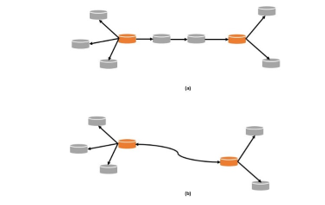
Fig. 2 The depiction of (a) ‘in-band’ and (b) ‘out-band’ wormhole attack.
The wormhole attack can be categorized into two classes based on the wormhole link formation. In the ‘out band’ wormhole [21], two external nodes are deployed with higher communications and computational power than deployed sensor nodes. This kind of attack is hard to establish due to the requirement of the special hardware. In this case, the adversary connects two separate regions of the network using a directional antenna or wired link. Similarly, in the ‘in band’ wormhole, the adversary compromises at least two legitimate nodes from the different zone of the network. One of these is usually located close to the base station so that it could disguise its adjacent nodes by advertising fabricated routing information. In contrast to ‘out of band’ wormhole attack, adversary uses packet encapsulation technique to create wormhole node rather than a directional antenna or wired link [9]. In this circumstance, two compromised nodes are connected through several legitimate nodes between them.
Once the wormhole link is functional, one of the colluding nodes transmits the data packets, collected from the one part of the network, towards another malicious node. The other malicious node broadcasts those received packets into its radio range [22]. The wormhole node influences those nodes, who normally multiple hops away from it, to send data packets via wormhole by convincing them that they are few hops away from the base station [23]. In the other words, due to the high-speed wormhole link, the received data packets (by wormhole nodes) would travel faster from one part of the network to another part of the network than a usual multi-hop route. This illusion would disrupt existing packet routing mechanisms.
At the initial stage, wormhole node eavesdrops or captures the packets passing through it for further analysis and retransmits them to another wormhole node. When the wormhole attack begins, malicious nodes do not know about the cryptographic keys are being used in the network. If this malicious node starts dropping the packets without knowing the content of the packets, the target of compromising the integrity and confidentially would not be achieved. On the other hand, the dropping of the packets might rise suspicion of those nodes who have relayed the packet through wormhole node. Therefore, there is a chance of being detected as a malicious node in the network. In fact, Wormhole node tries to place itself in most of the route without revealing its identity. However, the initial phase of wormhole attack is called hidden wormhole attack [20]. In the hidden mode of attack, the wormhole does not appear in the routing table. Still, wormhole node is able to establish the denial of service (DOS) [24] attack by dropping packets in the hidden mode of attack.
Once the wormhole node breaks the encryption technique by analyzing the recorded packets, then the aggressor takes the attack to the new level. In the active mode, the malicious node takes part in the routing mechanism as legitimate node [20] and starts modifying or dropping the packets passing through it [4]. In some cases, wormhole node drops the selected or critical packets to interrupt the usual operation of the network [21].
2.1. The impact of wormhole attack:
Wormhole attack is considered as server threats for routing protocols of WSNs. This attack usually occurs in the network layer and immune to encryption techniques. The wormhole attack is able to degrade the performance of the routing protocol and compromises the integrity and confidentiality of the data packets traveling throughout network [25]. Once wormhole nodes get the access to the network, the adversary can drop the packet selectively or delay the transmission of critical packets for the system in order to destabilize the system performance [21]. The aggressor tries to establish the denial of service attack (DOS) and attempts to compromise the integrity and confidentiality of the network.
During the active mode of this attack, the malicious nodes become the sinkholes [4]. However, other nodes around wormhole send data packets without aware of the fact that they are the victims of the wormhole attack. Hence, a significant amount of data traffic is passing through the malicious node and attacker can control and monitor the packets without having multiple observation points in the network. Some literature also suggests that wormhole node also lessens the throughput of the network by the selective dropping of the packets [4]. Furthermore, wormhole node also can turn on and off the wormhole link randomly [4]. This event creates instability in the routing service and causes a significant amount of control packets flow throughout the network.
In general, the routing protocol of the wireless sensor network can be categorized into two classes, such as ‘pro-active’ routing protocol and ‘on-demand’ routing protocol. Routing updates are transmitted periodically in the pro-active routing protocol, whereas on-demand routing protocol searches the route to a specific destination when it is necessary. However, the wormhole attack is successful to invade the network accessibility for the both class of wormhole attack [26]. Some literature on wormhole attack mentions that two wormhole nodes are able to attract more than 50% data traffic towards them directed to the base station[6][27].
3. Related works
As the wormhole attack can be launched from legitimate nodes and relays the valid packets into the network; therefore, it is reasonably difficult to detect it from the infected network. Furthermore, lightweight cryptographic solutions are incorporated into most of the routing protocol to prevent false data packets injection into the network. As the legitimate nodes are compromised by the adversary and the wormhole node doesn’t change the packet’s content at the initial stage, so the wormhole node easily passes the cryptographic test. The wormhole attack is a simple task to launch, but very difficult to identify. Many researchers have been working on this field to develop efficient wormhole detection schemes based on the geographical locations, transmission time, connectivity graph, neighborhood counts and radio fingerprint.
3.1. Distance consistency based approach:
Most of the researchers in this field try to detect the wormhole attack by distance bounding techniques. In these approaches, two communicating nodes are allowed to determine the distance between them; based on message traveling time information, transmission time information, and geographical information. Sometimes sensor nodes are equipped with specialized hardware like the directional antenna, GPS, ultrasound[8] to measure the distance between two adjacent sensor nodes. However, these schemes are considered impractical due to the addition of the special hardware and their performance in the sparse sensor network. These schemes may not perform well in the presence of ‘out of band’ wormhole nodes.
3.2. Time information based solutions:
The most popular detection methods of wormhole attack use the packet traveling time between two consecutive nodes as a detection attribute. Most of the cases, the data packets traveling time is calculated from the measured round trip time (RTT) [28-31], the authors proposed RTT based solutions to confront against wormhole attack. In [32], delay per hop is determined by measured RTT whereas, for each successive hop, RTT is measured to detect wormhole attack [33]. In these schemes, the distance between two adjacent nodes is measured using RTT and determine if the two communicating sensor nodes are apart by the valid possible distance. If the measured RTT is higher than a defined threshold value, the presence of wormhole node will be declared. However, the RTT based solutions require the cooperation of the sensor nodes on the path and don’t work properly on the DSR[34] and DSDV routing protocols [35-36]. These RTT based solutions may not perform well if the wormhole is created by protocol deviation. The wormhole nodes forward the packets without waiting for the certain time in order to reach the destination earlier than legitimate multiple hop path. Beside this, in the ‘out of band’ wormhole attack, the wormhole nodes use the high-speed low latency link for transferring packets between them. In this type of attack, data packets reach to another wormhole node more quickly than ‘In-band’ wormhole attack. In fact, the time required to forward the packets to another wormhole node is significantly reduced in ‘out of band’ wormhole attack. Therefore, the performance of RTT based detection scheme is in question with the presence of ‘out of band’ wormhole attack. Some works of literature [37] also suggested that the RTT based detection scheme cannot detect ‘active’ mode of wormhole attack and may not detect wormhole attack in the sparse sensor network.
In [38], the authors proposed a detection scheme based on neighborhood count and RTT. The authors considered the two facts. First, as the malicious nodes establish the new link in the network, so the neighbors around the malicious node increases significantly. Second, the measured RTT between two malicious nodes increases significantly in a similar fashion. However, these proposed solutions may not detect ‘out of band’ wormhole attack from the infected network.
In [37], the authors proposed a detection scheme based data transmission time of each successive hop in a route assuming that the wormhole nodes are in hidden mode. In this scheme, the data transmission time of each successive hop is calculated from the measured RTT. All sensor nodes in the route transmit the recorded transmission time to the source. The source is solely responsible for checking if there is any wormhole node exist in the route. This scheme may perform poorly in the sparse sensor network. In fact, the performance of this scheme may be degraded when malicious nodes use high-speed communication channel.
3.3. Special Hardware-based scheme:
The directional antennas are incorporated with sensor nodes for adding access restriction [6,39-41] and finding legitimate neighboring nodes in the network. The entire communication region of a sensor node is divided into several zones. Moreover, each zone is defined by a directional antenna. When a sensor node receives the signal first time from its peering sensor node, then the probable location of the sender in terms of the zone is determined by the directional antennas. According to the authors, if a sensor node sends a packet from a particular zone, the recipient will get the signal from the opposite direction (zone). After that, the recipient sensor node verifies the legitimacy of the sender through receiving direction of the packet from unknown sensor nodes. The recipient node also cooperates with its neighbors to find out whether this node is known to other legitimate neighboring nodes or not. The incorporation of directional antennas to each sensor node makes this scheme expensive and inappropriate for practical deployment.
Another protocol named SECTOR was introduced in [29], that mostly depends on special hardware. The main concept of this detection scheme is to measure the distance between two communicating nodes based on the data transmission speed. The proposed model does not need any clock synchronization and geographical information of communicating nodes. In this algorithm, the mutual authentication with distance bounding (MADB) protocol [42] was implemented to measure the distance between nodes at the time of the encounter. According to the authors in [42], the proposed scheme permits one node to measure the mutual distance between two nodes and compares with maximum possible upper bounding distance. In this scheme, each node is incorporated with the special device that can give feedback to the sender without any delay. Initially, a node sends the one-bit challenge to its neighbors before sending any packets. Then recipient node responds back through a special device to the sender at the time it receives the one-bit challenge. When the sender transmits the one-bit challenge to a node, it turns on the clock and measures the time till it gets the response back from that node. After that, the sender estimates the mutual distance based on the measured time assuming that the data transmission speed is as same as the speed of light. However, in the [30], the authors slightly modify the schemes described in [42]. In [30], both parties are allowed to measure the mutual distance and validated the authenticity of the adjacent nodes around their communication range. The addition of the special device to each sensor node makes this scheme expensive and inappropriate for practical deployment.
3.4. Geographical information-based schemes:
In [43] and [7], the author proposed a detection scheme that assigns a maximum traveling distance to each data packet. The authenticity of a data packet is ensured by using the concepts of geographical and temporal packet leashes that would help to minimize the effectiveness of the wormhole nodes in the network. In the geographical leash (GL), when a sender sends packets to any sensor node, the sender node incorporates sending time and its own location information to the packet. When the recipient node receives the packet, it will estimate the approximate distance between the sender and receiver based on the geographical leashes. The temporal leash includes the maximum lifetime to each packet. In temporal leash (TL), a sender adds either transmitting time or expiration time of packet so that the recipient can verify if the packet has made a journey too far based on maximum transmission speed and time. A predetermined time threshold is set between any two neighbors based on their position in the network. For a specific two neighboring nodes, the data packet would be discarded if it violates the time boundary set by these specific nodes. This scheme can perform better if strict time synchronization and the additional device like GPS are provided. Beside this, this proposed scheme may be performed poorly when the wormhole node is in active mode.
3.5. Trust Based Solutions:
Trust information of neighboring nodes is used as an attribute to detect wormhole attack in the WSN. Each sensor node monitors the data packet forwarding pattern of its neighbors and rates them accordingly. In the trust base scheme, a sensor node selects the most trustworthy path to reach the destination based on the trustworthiness of its neighbors. In this scheme, the researchers consider the fact that the wormhole node drops all the received packets coming from its adjacent nodes. It is expected that the system would rate the least trust level to the malicious nodes. By using this trust level scheme, the wormhole node can be avoided during the selection of a path to the destination. This also helps to reduce the effectiveness of the wormhole nodes in the infected network. The source node would forward the packets to the neighbor which possess maximum trustworthiness.
In [44], a new detection scheme was proposed to detect wormhole attack in the network based on both time and trust. In this scheme, both data travel time and trustworthiness of the sensor are used as potential attributes to detect the malicious nodes from the infected network. These two modules of this proposed scheme run in parallel. Here, the time-based module works in three stages. Firstly, each sensor node identifies its neighbors and update the neighbor list accordingly. Secondly, each node finds the best path toward the base station based on the trustworthiness of neighbors. Finally, the proposed algorithm determines the presence of the wormhole nodes in the selected path. According to the authors, the malicious nodes deceive the time-based solutions in many ways. Hence, the trust-based model is incorporated with the time base scheme. In this scheme, a sensor node monitors the neighboring node continuously and select the best route to the destination based on the rating.
Another trust based wormhole attack detection scheme was proposed in [45].To execute the model, the deployed sensor node must operate in a particular mode, named as ‘promiscuous mode’. This trust-based scheme is applied to the DSR protocol and inherent features of DSR routing protocol are used to measure the trust level of the neighboring nodes. Here, the algorithm must be executed in each sensor node and each node must measure the trust level of its neighboring nodes by monitoring the packet transmission pattern stated by the system. The source node verifies in several stages whether the forwarding node passes the IP packets or not through the sequence of integrity check. If the neighboring node for a particular source forwards all the packets, the trust level of the node would be increased. Similarly, if the opposite happens, the trust level of that node would be decremented.
The success of this module lies on the packet dropping criteria of the malicious nodes. However, the wormhole nodes do not drop packets in the hidden mode of this attack. Hence, the trust base detection model is not capable of detecting the hidden wormhole attack. On the other hand, each node monitors the packets forwarding pattern of its neighbors. As we know, sensor nodes have some constrained-on power and energy resources. It would be a burden for the system which leads to excessive energy dissipation of the nodes.
3.6. Graph-based solution:
Multi-dimensional scaling-visualization of the wormhole (MD-VOW) [46], was proposed based on the graph theory. The multi-dimensional scaling analysis of the constructed connectivity graph was used as an analysis tool to detect malicious node in the network. For the static sensor network, the connectivity graph is not supposed to change frequently. Hence, the authors have considered the fact that the presence of malicious nodes introduces the anomalies in the connectivity graph. In the network connectivity based wormhole attack detection schemes, the positions of the neighboring nodes are estimated from the received signal strength (RSSI) by each node and send this information to the base station. By compiling the received information, the base station determines the network layout and compared with the current connectivity graph. Then the presence of the wormhole node can be detected if any forbidden structure is found in the constructed network layout. However, it is prone to the distance estimation errors, especially for the sparse network. The surface smoothing technique is applied to the constructed network layout graph to compensate distance error. This approach also causes a significant amount of control packets flow to the base station. Similarly, if the wormhole node is located in the sparsely populated area, then the wormhole attack may not be identified by this network visualization based algorithm.
3.7. Radio fingerprinting based scheme:
In [47], the authors explored the potentiality of the fingerprinting device as a tool to validate the legitimacy of the node in a wireless sensor network. Most important goal of this research is to extract the features from the radio signals, radiating from the nearby sensor nodes; by which the legitimacy of a node can be evaluated. In this research, each node has to be equipped with the radio fingerprinting device. The radio fingerprinting device captures the radiated radio signal from the nearby sensor nodes. After that, the fingerprinting device converts the radio signals into digital format. The transient part of the signal is located and the important features are extracted. After that, those extracted features are taken into account as fingerprints so that recipient sensor node can identify the neighboring node. The authors also implemented the incorporation of the radio fingerprinting device with a sensor node [47]. In this research, the authors also showed that the fingerprinting approach identified the nearby node while the message contents and the identification of the nearby devices were hidden. There are few issues are required to be investigated in this approach. The radio fingerprinting devices’ performance in a noisy environment, and in the mobile platform is in question. By using this detection method, only the ‘out of band’ wormhole attack can be detected. This proposed algorithm cannot detect ‘in-band’ wormhole attack as it can be launched from the legitimate node.
3.8. Neighborhood counts based detection scheme
No. of neighbors around a sensor node are used in [10-12,19] as detection attributes in the neighbor based detection scheme. In the centralized method, each sensor node finds the number of neighbors within its communication region and sends this information to the base station. As the distribution of the sensor node is known, the base station computes the hypothetical distribution of the number of neighbors along with the true distribution of the neighborhood counts. This process also creates a significant amount of control data packet flow throughout the network and leads to the unexpected energy dissipation of sensor node. This process is also used as secondary approach with the distance-based scheme. In another neighborhood count based approach [12], detector node takes the count of neighbors at the each site it visited. In this approach, ANN-based detection scheme may not able to detect the wormhole attack if the wormhole nodes are located in the sparsely populated area. Another important factor is that by this scheme, the probable location of the wormhole node cannot be identified. Some authors also use signal processing tool like Fourier transform, Discrete wavelet transform [48] and, variance fractal dimension [49] on the data series of the neighborhood counts. However, these proposed algorithms only work on the acquired data series while deployed sensors are distributed uniformly. However, these schemes may not able to locate the probable location of the wormhole node.
4. Artificial neural Network (ANN)
The Artificial Neural Network (ANN) is a network based stochastic learning model that has evolved from the study, characteristics, organization, and decision-making ability of the unit cell of a human brain called a neuron [19]. In other words, it aims to imitate the most simplified and basic function of the human brain. Analogous to the unit cell of a human brain, an ANN contains several interconnected information processing units, called a neuron, learning the underlying process of the data samples presented to the network. The significant phenomena of ANN are the ability to estimate the non-linear complex relationship between inputs and outputs without any prior knowledge of dataset like a black box. ANN is usually observed as a model of interconnected neurons that maps the input and outputs through information exchange among neurons[50].
Furthermore, in a multi-layer perceptron (MLP), there is an input layer, followed by one or more hidden layers, and an output layer [51]. In each layer, several neurons are employed, which are fully connected with other neurons of an adjacent layer, and they are connected to different random weight values. In other words, neurons are fully attached to the neurons of the following layer; but in the same layer, neurons are not connected with each other. The number of neurons in the output layer depends on the type of the problem that we want to solve by the ANN.
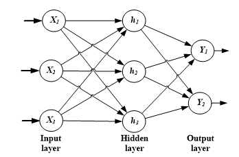
Fig. 3 The structure of an ANN.
4.1. Forward Propagation of the ANN:
Input features from the input layer are shared with an adjacent hidden layer through unidirectional branches[50]. Those input features are multiplied by random weights associated with the unidirectional branches; summed up, and passed through the activation function of the neuron (e.g. sigmoid function). The bias term is also added to each layer except the output layer to activate the artificial neurons. This bias term is also connected to the neurons of the adjacent layer with unidirectional branches associated with the weight values ( ) so that the summed inputs exceed the predefined threshold.
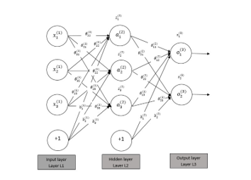
Fig. 4 Forward propagation of ANN
In the forward propagation, the output of each neuron of the prior layer is considered as the input to all neurons of the following layer. As shown in the Fig. 4, the three layers are connected with the weight value . represents the weight value going to the unit in layer and coming from the unit in layer . According to the Fig. 4, the net output of unit (including bias term) of the hidden layer ( is,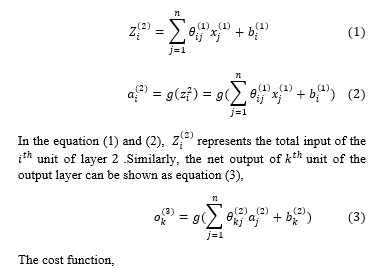
In the equation (4), refers to the average error occurred over training samples during the training procedure, and defines the number of neurons in the output layer.
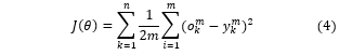
The transfer function of a neuron plays an important role in the training procedure. The purpose of the transfer function is to replicate the activation mechanism of the biological neuron. Usually, the net output of a unit in a layer is calculated from the net received input through the transfer function. The transfer function must be non-linear, continuous and differentiable at any point in order to apply gradient descent learning algorithm. There are several types of transfer function such as sigmoid function, hyperbolic tangent function, and rectified linear function. Some literature also suggests that the rectified linear function was found to accelerate the convergence rate of stochastic gradient descent due to its non-linear and non-saturating form. However, in our research, the sigmoid function was used as the transfer function of each unit in any layer (except input layer).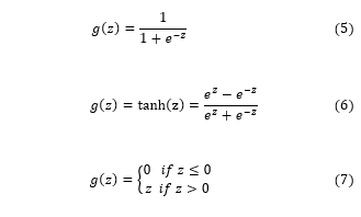
4.2. Back Propagation of the ANN
In the back propagation, the outcome of the output layer is compared with desired output. The error between the network output and desired output is measured and propagated backward to adjust the branch weights in order to minimize error that would occur due to the estimation of output. In other words, we minimize the cost or energy of the error function, by passing back the error occurred during the training phase. In the back propagation, the gradient descent algorithm is applied to learn the network parameters ( from the training set .
However, there are many ways to update the weights: batch mode, online mode. In the batch mode, each weight is updated once by the total error occurred in an epoch (i.e. after one training cycle). In contrast, in the online mode, a training sample is drawn randomly from the training set and passes through the network. The network parameters are modified times per training cycle if there are training examples in the training set. This online mode of weight updating is also known as stochastic gradient descent[50].
Let’s consider the multilayer feed forward network shown in Fig. 4. The impact of the change in the weight on error occurred in the output layer is,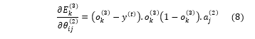
In the equation (8), represents the output of the unit of the output layer and refers to the desired output of a training example. Similarly, the impact of the change in weight ( , associated with bias and the neurons of the output layer, on error occurred in output layer is,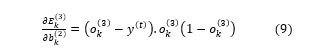
According to the above equations (8) and (9), the update formulas for the weights associated with output layer are given below.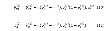
In the equations (10) and (11), refers to the learning rate of the network. Now, we can calculate the rate of the change in the error over the weight ( , associated with the input layer and the hidden layer shown in the equation (12).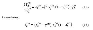
Similarly, impact of the changes in weights ( , associated with bias and the neurons of the hidden layer, on error occurred in output layer can be calculated as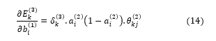
Therefore, according to the equations (12) and (14), the weights associated with input layer and the hidden layer can be modified by the following equations during the training procedure. ![]()
![]()
These weights adjacent procedure continues recursively until the network reaches either to the minimum tolerance level or maximum epochs at the training.
5. Support Vector Machine
The support vector machine (SVM) is one of the reliable and widely used supervised learning models that analyze the presented data samples to perform classification and regression analysis[50]. The SVM learns the given data samples, each sample marked with a specific class, builds a model that can assign a class to a new data sample. SVM learning model set a hyperplane in an optimum position in the data space so that Euclidian distance from the decision surface for all training data samples would be maximized. SVM has been emerged to provide the generalized performance to solve a wide range of classification and pattern recognition problems such as face detection, pedestrian detection, and text categorization etc.
Let’s consider a training data set, contains training data samples where and , represents the label of the data sample. The hyperplane in form of decision surface can be defined as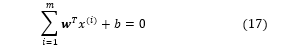
In the equation (17) and b represent a weight vector and a bias term that can be determined through the training process. Through these parameters , the decision surface places itself in the optimum position in the data space. As we know, the SVM places the decision surfaces in the data space in such way that it maximizes the geometric margin of all training data samples. In this circumstance, the optimization problem is 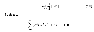
The concept of the Lagrange multiplier is implemented to solve this optimization problem with constraint boundary stated in the equation (19). Therefore, the Lagrange function is 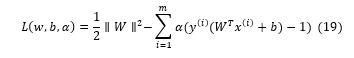
In the equation (19) is the multiplication factor and . If we differentiate the Lagrange function with respect to and ; then the optimization problem mention in the equation (18) can be formulated as 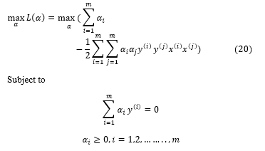
In the equation (19) is the multiplication factor and . If we differentiate the Lagrange function with respect to and ; then the optimization problem mention in the equation (18) can be formulated as 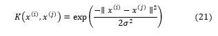
6. Non-linear Logistic regression
Logistic regression is a statistical model in which the category, from a predefined list of categories, of a new observation or data sample, is predicted, by estimating the probability of the class using a logistic function (e.g. email sorting). It is evolved from linear regression and designed to solve classification problems. That’s why, in some literature, it is referred as logistic classification[50].
Logistic classification can be shown as a special case of linear regression, but we can draw a distinct line between these two statistical models. In the linear regression, the predictor predicts the continuous value by a fitting curve to the given training input data samples [53]. In contrary, in logistic classification, a predictor learns how to classify the data through a training phase and predicts a discrete value for the corresponding new data sample. Like linear regression, the same decision boundary equation is used for logistic classification.![]()
Here, in the equation (22), represents a given input vector that contains input features. The refers to the model parameter that is required to be optimized by using the training input data samples. This decision boundary can be either linear or nonlinear that depends on the application of the logistic classification.
In logistic regression, a sigmoid function is used to measure the certainty level of the class that new observation or data sample belongs to. The main advantage of using sigmoid function is that it is continuous, differentiable at any point and monotonically increasing. The probabilistic interpretation can be done in a simple way; as the value of the in greater than 0.5, the predictor would be more certain about the class of the given data sample [54]. If the same cost function of linear regression is used, yields non-convex cost function. Consequently, special kind of the cost function is used in logistic classification to learn model from the training data which is convex.
denotes the cost function of the logistic classification with regularization term, where refers to the total training examples of a given training set, is the regularization parameter, represents the target output for training example, and represents the training example. There are two learning methods used in the training procedures: Gradient decent and Newton’s method. In this research, the newton’s method is applied as the learning model. Because it converges to the optimal solution within few iterations.
7. Propose detection scheme
The proposed algorithm is a network based approach, in which neighborhood counts are used as the detection feature to detect a wormhole attack.
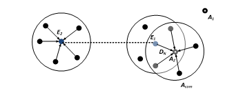
Fig. 5 Impact of wormhole attack on neighborhood count
A mobile sensor node, known as detector node ( ), is deployed in an area where sensor nodes could be uniformly or non-uniformly distributed. The detector node moves around this sensor field and collects a neighborhood count and the coordinate at each site it visited. When it reaches to the wormhole infected zone, the neighborhood population would increase abnormally sharply or abnormally lightly, depends on the sensor distribution and the position of the wormhole nodes. For instance, Fig. 5 shows the impact of wormhole nodes on the neighborhood counts. Let’s say, the detector node is moving spontaneously around the area where the sensor nodes are deployed. At the time , moves from a location to another location . Since the detector node collects the neighborhood count at each site, it transmits neighbor discovery message (NDM) to the adjacent sensor nodes within its communication range. According to the Fig. 5, the wormhole node also hears the broadcast as it is located in the transmission range of .Since wormhole node doesn’t read the content of the packet, it encapsulates and forwards the packets along the virtual tunnel to another malicious node . Furthermore, retransmits the received packets towards its neighbors. The neighbors of the distant malicious nodes respond back with valid neighbor ID (NID) through the wormhole link. After that, unicasts the received responses to the originator, . compels to think that the responses have come from the sensors located within its radio ranges. Though some of those responses have traveled long distant within the network. That’s how the neighborhood counts from the infected zone increases sharply due to the wormhole node shown in the Fig. 6. This may be true for uniform sensor distribution.
As we know, the sensor density in the non-uniform sensor distribution is inconsistent over the area. If the wormhole nodes are placed in the sparsely populated area, then the number of neighbors would not increase abruptly or lightly as expected. In this circumstances, it would be difficult for ANN based detection scheme to detect wormhole attack based on the collected neighborhood counts (also true for the sparse network).
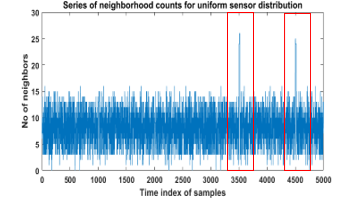
Fig. 6 The series of neighborhood count (Uniform sensor distribution)
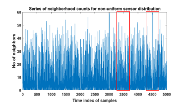
Fig. 7 The series of neighborhood count (Non-uniform sensor distribution)
Sometimes the neighborhood counts taken from the infected zone are same as, or far smaller than the counts taken from the non-infected zone shown in the Fig. 7. In this case, the ANN-based detector may suffer to distinguish between positive and negative data samples. Therefore, another detection feature along with neighborhood count is required in order to detect wormhole attack from the infected network (either uniform or non-uniform) more precisely and confidently.
In this paper, we introduce a new detection feature called ‘average residual energy pattern of the neighbors (AREPN)’. As we know, wormhole nodes circulate false route information into the network that the base station is multiple hops away from the wormhole nodes. Therefore adjacent sensor nodes of the wormhole get influenced and transmit their data packets to the base station through wormhole nodes. However, the wormhole nodes force them to hand over the collected data packets to one of the wormhole nodes. That means the wormhole nodes receive more data packets after the base station and its neighbors. Now, the question is how the wormhole nodes get those data packets coming from the adjacent nodes. Apparently, the data packets are coming through its neighbors.
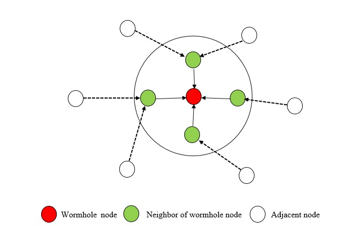
Fig. 8 Impact of wormhole nodes on adjacent nodes.
More packets arrive at the wormhole node means, more packets have been received and transferred by its neighbors. As we know, a node dissipates a significant amount of energy due to the transmission and reception of the data packets. Since the wormhole nodes are getting the numerous data packets from the adjacent nodes, so the neighbors of the wormhole nodes are also losing energy more quickly by retransmitting packets intended for the wormhole node. Now it can be said that the sensors located in the infected zone lose more energy than other nodes located in the non-infected zone.
In our proposed scheme, the detector node broadcasts NDM to the adjacent sensor nodes at each site it visited. The adjacent nodes reply back by transmitting a data packet incorporating valid NID and information of residual energy. By this way, is able to calculate the number of neighbors and average residual energy of the neighbors (AREPN). captures this evidences as a two-featured sample and stores it. It is expected that AREPN taken from the infected zone is much smaller than the AREPN taken from the non-infected zone. As we know, the adjacent nodes of the base station dissipate energy quicker than the normal node. That’s why, doesn’t cover a certain geographic area based on the location of the base station. Once the mobile node reaches close to the base station, it transfers all the collected samples for further analysis.
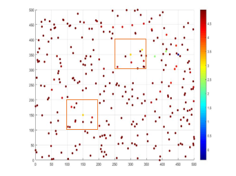
Fig. 9 Wormhole infected network.
As shown in the Fig. 9, the sensors of the wormhole infected zone lose energy (red marked box) more quickly than the non-infected zone. In that case, the initial energy of each sensor node is 5 units.
The performance of an artificial neural network highly depends on the method of training and the dataset containing potential features. The Base station gathers (by the help of the detector node) a data set consists of data samples. In this first half, gathers two featured data samples ( from the non-infected zone which are called negative data samples. Similarly, the same amount of data samples is collected from the wormhole infected zone, known as positive data samples. After that, those two types of data samples are mixed up randomly so that training can be performed without any bias. Then, data samples ( are drawn from the and stores in a training dataset . At the same time, rest of the data samples ( are stored in to evaluate the learning performance of the trained neural network.
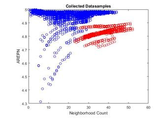
Fig.10 Collected two featured data samples by D_N (red marked samples are positive data samples) .
| Proposed Algorithm: |
- Collect two featured negative data samples from the non-infected zone
- Collect two featured positive data samples from the wormhole infected zone
- Store the both type of data samples in which consists of data samples
- Select data samples from and store in where
- Rest of the data samples are stored in where
- Train the neural network with the data set and appropriate network parameters up to epochs
- Test the neural network by using the samples of
- If output for a specific sample , then this sample represents wormhole attack and probable location of the malicious node are identified.
- If output for a specific sample then this sample doesn’t represent wormhole attack
- Update by for further training
- Reset and update with new data samples gathered by
Furthermore, data samples of are fed into the input layer of the ANN. The training procedure is performed repeatedly until it reaches a predefined maximum number of training cycles i.e. epochs. The testing procedure involves checking the learning progress of the ANN-based detector. In the testing part, each data sample passes through the trained neural network. If the output for a specific data sample is greater than 0.5, then this sample represents wormhole attack. Since, stores the coordinate of the locations along with the two featured data samples, so the probable position of the wormhole node can also be identified by the detection scheme.
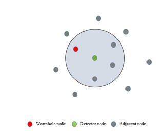
Fig. 11 Probable location of a wormhole node
After that, is updated by the for further training. This would minimize the error level that has achieved in the training phase. The entries are cleared up and updated with new data samples collected by the in real time.
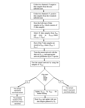
Fig. 12 Flowchart of the ANN-Based proposed algorithm
8. Simulation and results
In this section, extensive research experiments are conducted under various network scenarios to assess the effectiveness of the proposed algorithm in detecting wormhole attack from the affected sensor network. The first phase of the experiments is conducted to see if the proposed scheme is able to classify the malicious data samples that represent wormhole attack. Furthermore, we evaluate the performance of the detection scheme in terms of detection accuracy, false positive rates, and false negative rates. In the second phase, the efficacy of the proposed algorithm is explored considering single featured data samples and two featured (i.e. the number of neighbors and AREPN) data samples. As the energy dissipation of the sensor node depends on the routing protocol; hence, the proposed algorithm is also tested considering ‘On demand’ based routing protocol (AODV) and cluster based routing protocol (LEACH). Afterward, we record and analyze the efficacy of the proposed algorithm in detecting wormhole attack from different sensor distributions. Finally, the performance of the proposed algorithm is compared with the performance of other machine learning technique based detection schemes like support vector machine (SVM) and regularized non-linear logistic regression (LR). In addition, all experiments have been performed in MATLAB 2015a.
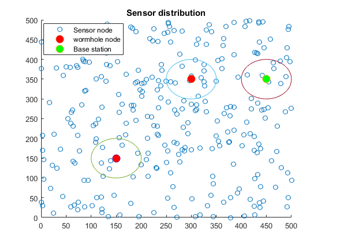
Fig. 13 The depiction of the simulation set up (uniform sensor distribution)
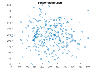
Fig. 14 Non- uniform sensor distribution (Gaussian)
In the simulation, 300 sensor nodes are distributed (uniform or non-uniform) within the square field of . The deployed sensor nodes and the base station are static in nature. Each sensor node has the communication resources of which they use to communicate with the adjacent sensor nodes. Radio range of each sensor node equals to . Initially, each sensor node has five (05) units of energy that would be used in sensing and transferring packets. A detector mobile sensor node, is deployed as a mobile observation point of the network. The basic task of the is to collect neighborhood counts and AREPN of neighboring population at each site it visited within this deployed area. The radio range of the detector node is same as deployed sensor nodes. We assume that the detector node is fully aware of its position, the boundary of the targeted area, and any obstacles in the area that may restrain its movement. A pair of wormholes node is placed at the locations , and . Random waypoint model is implemented in the simulation as the mobility model for the .Similarly, the base station is positioned at a location of .In these experiments we only consider the data communication between a node to the base station. Moreover, the experiments have been conducted on thirty (30) different instances for each sensor distribution (e.g. uniform sensor distribution) in order to get valid (average) performance matrices of the proposed detection scheme.
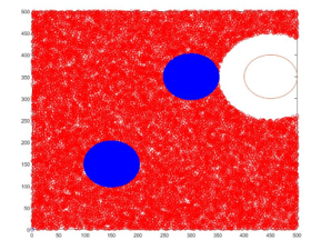
Fig.15 The location visited by the Dn ( red ,blue and white indicate non-infected zone, infected zone and the area not covered by Dn).
In this simulation, the detector node collects two featured data sample (i.e. number of neighbors and AREPN) at each site it visited. For each instance of each sensor distribution (uniform or non-uniform sensor distribution), the detector node, collects 50000 data samples from deployed area in which 25000 samples are negative data samples, and 25000 samples are positive data samples. The collected data samples are stored at the in the base station. After that, 49000 randomly selected samples are stored in the for the training purpose. Rest of the data samples is used to test the learning performance of the proposed detection scheme.
8.1. The performance of Proposed ANN based detection scheme:
A multi-layer, feed forward network (with back propagation algorithm) is implemented for the experiments. The input layer contains one or two neurons considering the type of data samples (one featured or two featured) used to train the network. Moreover, the hidden layer consists of 100 neurons and the output layer has only one (01) neuron. We used a sub data set, comprised of 49000 randomly selected data samples from for training collected by .
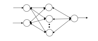
Fig. 16 The structure of the ANN for two featured data samples
At first, the neural network was trained by the single featured the training examples from and evaluated learning performance of ANN by the rest of the data samples stored in the . After that, two featured training samples are fed into the neural network and acquired results are compared with the results obtained by using single feature data samples. During the training period, the minimum error tolerance level is set to . The Table 1 represents the parameters which are used during the training phase.
- Parameters used for ANN.
| Parameter | Value |
| No of attributes | 2 |
| No of Data points (training) | 49000 |
| No of Data points (testing) | 1000 |
| Architecture (for one feature) | [1,100,1] |
| Architecture (for two features) | [2,100,1] |
| Performance | 0.00001 |
| Learning rate, α | 0.001 |
| Epoch | 500 |
| CPU time (for one instance) | 2.17 mins |
In the testing phase, the test data set, is fed into the input layer. Then the output of the ANN based model is observed if it could detect the existence of wormhole attack in the given network. Fig. 17 shows that, the ANN based wormhole attack detection scheme can classify the samples that represent wormhole attack from the both single featured and two featured data samples successfully
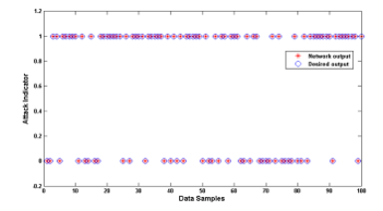
Fig. 17 Classification of wormhole attack
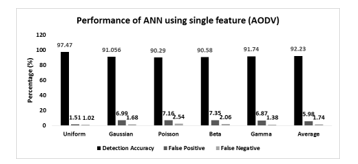
Fig. 18 Performance of the ANN-based detection scheme using single featured data samples (AODV)
Fig. 18 shows the performance of the ANN-based detection model in detecting wormhole attack using single featured data samples (i.e. neighborhood count) when the network uses AODV routing protocol. In this graph, the highest detection accuracy is recorded as 97.47% when sensors are distributed uniformly in the square field, whereas the lowest detection accuracy is measured 90.29% for poisson sensor distribution. Furthermore, detection accuracy for Gaussian distribution is almost same as the gamma distribution. Accordingly, 91.056%, 91.74%, and 97.873% detection rates are measured for Gaussian, Gamma, and Beta sensor distribution. However, the average detection accuracy is calculated as 92.23%. The false positive rate and false negative rate entirely follow the same trend of detection accuracy. The lowest false positive rates and false negative rates are measured for uniform sensor distribution. The average false positive rates and false negative rate are accordingly 5.98% and 1.74%.
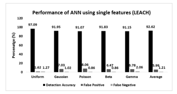
Fig. 19 Performance of the ANN-based detection scheme using single featured data samples (LEACH)
Fig. 19 shows the results obtained by applying single featured data samples on ANN based detection model considering LEACH routing protocol. It is observed that this algorithm performs better for uniform sensor distribution compares to non-uniform sensor distribution. 97.63% detection accuracy, 1.62% false positive rate, and 1.23% false negative rate are achieved for the uniform sensor distribution. After that, it has performed better for Gaussian sensor distribution among all non-uniform sensor distributions. The detection accuracy, false positive rate and false negative rate for Gaussian sensor distribution are 91.95%, 7.03% and 1.02% accordingly. The similar trend in detection accuracy is observed for Poisson, beta, and gamma sensor distribution. However, considering all the sensor distributions, the false negative rates are lower than the false positive rates. The average detection accuracy and false positive rate for all sensor distributions are accordingly 92.62% and 5.99%.
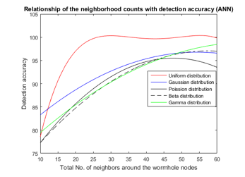
Fig. 20 The relationship between neighborhood count and detection accuracy (ANN)
Fig. 20 represents the relationship between the neighborhood counts and the detection accuracy. Undeniably, the detection accuracy of the proposed algorithm (considering single featured data samples) increases as the total number of neighbors around wormhole nodes increase for all sensor distributions. The detection accuracy of the system has a non-linear relationship with the total number of the neighbors around the wormhole nodes. For the uniform sensor distribution, we can model this relationship as degree polynomial. For the other non-uniform sensor distribution, the relationship can be modelled as .It means that the proposed scheme may not perform well considering single featured data samples if the wormhole nodes are located in the sparsely populated area in the network.
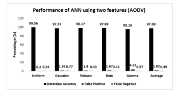
Fig. 21 Performance of the ANN-based detection scheme using two featured data samples (AODV)
The two featured data samples are applied to the ANN-based detection scheme. Like prior, the performance of the ANN is evaluated considering both AODV and LEACH routing protocol. Fig. 21 presents the performance of the ANN-based model considering two featured samples and AODV routing protocol. The proposed algorithm gives a better performance to detect the wormhole attack for the uniform sensor distribution. 99.56% detection accuracy, 0.2% false positive rates, and 0.24 % false negative rate are achieved for the uniform sensor distribution. For all non-uniform sensor distribution, the detection accuracy varies in between 95% to 97%. In this circumstance, the average detection accuracy and false positive rate for all the sensor distributions are 97.69% and 1.82%. Most importantly, the detection accuracy, considering all sensor distribution, is significantly increased for the application of the two featured data samples.
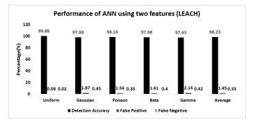
Fig. 22 Performance of the ANN-based detection scheme using two featured data samples (LEACH)
As shown in the Fig. 22, the performance of the ANN-based detection scheme improves significantly considering LEACH routing protocol and the application of two featured data samples on the ANN. Evidently, the ANN-based model performs better for the uniform sensor distribution compares to all non-uniform sensor distribution. The highest achieved detection accuracy for the uniform sensor distribution is 99.88%. The detection accuracy for the non-uniform sensor distributions fluctuates from 97.43% to 97.98%. Furthermore, the lowest false positive rates and false negative rates are achieved for the poisson sensor distribution which is 1.54% and 0.35% respectively. In this circumstance, the average detection accuracy, false positive rate, and the false negative rate for all the sensor distribution are accordingly 98.23%, 0.45%, and 0.33%. In summary, the application of the two featured data samples on the ANN enhances the performance of the proposed scheme for both AODV and LEACH protocol.
A. The performance of the SVM-based detection scheme
For the different sensor distributions, one and two featured training examples are applied to the SVM accordingly. The average result of detection accuracy, false positive rates, and false negative rates are calculated to measure the efficacy of the SVM-based algorithm for all network scenarios. The Table 2 represents the parameters which are used during the training phase.
- The parameters used for SVM
| Parameter | Value |
| No of attributes | 2 |
| No of Data points (training) | 49000 |
| No of Data points (testing) | 1000 |
| Kernel | Gaussian |
| Sigma | default |
| Tool | MATLAB |
| CPU time (for one instance) | 3.17 mins |
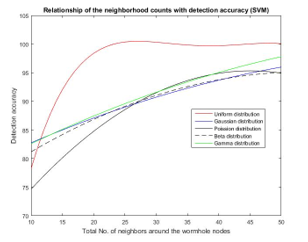
Fig. 23 The relationship between the neighborhood count and the detection accuracy (SVM).
Fig. 23 represents the relationship between the counts of neighbors around wormhole nodes and the detection accuracy considering one featured data samples applied to the SVM-based detection scheme. Like the previous case, the detection accuracy follows the non-linear relationship with the total number of neighbors for all sensor distribution. As the neighborhood count increases, the detection accuracy of the SVM-based algorithm also increases. Similar to the ANN-based detection scheme, it may suffer to detect wormhole attack if the wormhole nodes are placed in the sparsely populated area.
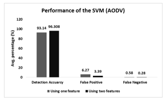
Fig. 24 Performance of the SVM-based detection scheme (AODV).
Fig. 24 shows that the performance of the SVM-based algorithm when the network uses AODV as the routing protocol. According to the Fig. 24, SVM-based detection scheme gives better the performance considering two featured data samples like the ANN-based model. SVM-based algorithm reaches approximately 96.30% on an average for all sensor distribution. Similarly, it achieves lowest false positive and false negative rates for two featured data samples which are 6.27% and 0.58% approximately. Using two featured data samples, the performance of the SVM-based algorithm enhances around 3.39%.
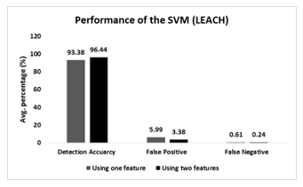
Fig. 25 Performance of the SVM-based detection scheme (LEACH).
Fig. 25 shows the performance of the SVM-based detection scheme considering LEACH protocol. Similar kind of trend in detection accuracy, shown in Fig. 24, is observed for the LEACH protocol. Like Fig. 24, SVM-based detection scheme performs better with the two featured data samples. It achieves averagely 96.44% detection accuracy for all sensor distribution, whereas, 93.38% detection accuracy is measured for the one featured data samples. In this case, the detection accuracy increases approximately 3.27% for the two featured data samples. Inversely, the false positive rates and false negative rates declined significantly for the two featured data samples.
B. The performance of the non-linear logistic regression:
Non-linear logistic regression (LR) algorithm is used to measure the performance on this classification problem and compare its outcomes with the proposed algorithm. Table 3 shows the parameters which are used during the training phase of the non-linear logistic classification algorithm.
- Parameters used for logistic linear classification
| Parameter | Value |
| No of attributes | 2 |
| No of Data points (training) | 49000 |
| No of Data points (testing) | 1000 |
| Iteration | 07 |
| Regularized parameter ( | default |
| Learning method | Newton’s methods |
| CPU time (for one instance) | 3.17 mins |
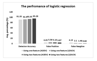
Fig. 26 Performance of the LR.
Fig. 26 represents the overall performance of the LR to detect the wormhole attack considering one featured and two featured data samples. According to the Fig. 26, LR based detection scheme performs better with two featured data samples when the network uses LEACH as the routing protocol. The detection accuracy reaches to 95.28 % considering two featured data samples. In this case, lowest false positive rate and false negative rate are achieved for the LEACH routing protocol, which is 3.87% and 0.82% respectively. Most importantly, this LR based detection scheme gives better performance with two featured data samples like ANN or SVM based detection scheme.
C. Performance comparison
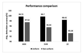
Fig. 27 Performace analysis on the uniform and the non-uniform sensor distribution.
Fig. 27 represents the performance of the detection schemes on the uniform and the non-uniform sensor distributions considering two featured data samples. Clearly, for the uniform sensor distribution, three (03) detection schemes achieve higher detection accuracy in contrast to the non-uniform sensor distributions. As the sensor density of the area is uniform; the neighborhood counts increase significantly with the presence of the wormhole nodes in the network. In contrary to the non-uniform sensor distribution, the neighborhood counts increase slightly or significantly depends on the position of the wormhole nodes in the network. Sometimes the neighborhood counts are smaller than the count taken from the wormhole non-infected zone (wormhole nodes can be placed in the sparsely populated area in the network). Since the uniform sensor distribution has consistency in the node density, the total neighbor population of the wormhole nodes is much smaller than the total neighborhood counts in non-uniform sensor distribution. As the neighbors of the wormhole nodes are the only way to reach the wormhole nodes; therefore, the neighbors of wormhole nodes in uniform distribution dissipate more energy than the neighbors of the malicious node in non-uniform sensor distribution. Hence, positive data samples are easily distinguished from the presented data set. That’s why the detection accuracy of these schemes is much better for uniform sensor distribution.
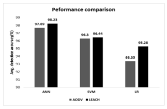
Fig. 28 Performance comparison among ANN, SVM, and LR.
If we analyze the performance of the three detection schemes (shown in the Fig. 28), ANN outperforms SVM and LR in detecting the malicious samples that represent wormhole attack considering both AODV and LEACH routing protocol. ANN achieves 97.69% and 98.23% detection accuracy respectively for AODV and LEACH routing protocol. SVM based detection scheme performs better than LR based detection scheme (achieves approximately 96% detection accuracy) in view of AODV and LEACH. Considering LEACH routing protocol, the LR based detection scheme attains 95.28% detection accuracy which is the lowest among all the detection schemes. As we know, the performance of the machine learning techniques highly depends on the dataset. In this case, ANN distorts the two featured data samples in the higher dimension better than other two machine learning techniques; and efficiently put dynamic decision surface in between positive and negative data samples. That would help the ANN-based detection scheme to gain highest detection accuracy.
Another important observation of this research is that the three detection schemes give better performance in classifying positives data samples for LEACH protocol. In the cluster based routing protocol like LEACH, a node is nominated as a cluster head among the members of a cluster for a specific round of data transmission to the base station. Once the cluster head is selected, other members send their data packets to the cluster head. Afterward, selected cluster head transfers the data packets to the base station. For the next round, a new member is randomly chosen as cluster head from the other members who is not selected as cluster head before for any round. However, wormhole node manipulates the cluster head selection process in a particular cluster of nodes. Furthermore, the ‘in-band’ wormhole node can be selected as a cluster head. If it happens, the wormhole node gets a bunch of data packets easily from the other members through its neighbors. As we know, wormhole nodes create shortcut path to the base station in the network. Therefore, the cluster head is deceived throughout the data transmission process to the base station. If wormhole nodes are placed in two different clusters, the members of the cluster may also be deceived while they are selecting closest cluster head to transmit their data packets. Hence, the neighbors around wormhole node dissipate more energy in LEACH compared to AODV. The extra dissipation of the energy reflects in the feature called AREPN collected by detector node. That would help in separating the positive data samples and negative data samples when two featured data samples are presented to the detection schemes.
9. Conclusions
Wormhole attack is one of the detrimental network layer attacks for wireless sensor networks. This thesis presents a novel detection model based on neighborhood count and AREPN using an ANN for wireless sensor networks. The goal of this proposed detection scheme is to detect wormhole attacks (In-band, out of band, hidden or active mode of wormhole attack) with higher precision and accuracy, especially in a non-uniform network environment. The experimental results confirm that the proposed detection scheme is able to identify the existence of the wormhole node without requiring any special hardware both in uniform and non-uniform sensor distribution. Another important aspect of this detection model is it doesn’t increase the significant amount of network overhead flow throughout the network. The simulation results also validate that our ANN-based approach performed better than SVM or LR based detection scheme. This ANN based detection scheme achieves around 99.72% (average) and 97.52% (average) accordingly for uniform and non-uniform sensor distribution. Most significantly, the probable location of the wormhole node can be identified by this scheme. Future works are required to enhance the performance of the detection scheme and to investigate in different directions so that we can evaluate the efficacy of the proposed detection scheme perfectly.
Proposed future works are noted as follows.
- Nowadays, deep neural networks and convolutional neural networks are used to enhance the performance internet threat detection schemes. We want to apply this advanced machine learning algorithms on the acquired data set to evaluate their performance. After that, we will compare the results with the Proposed ANN based scheme.
- In this research, the relationship between detection accuracy and the total count of neighbors around wormhole nodes is investigated. In the future work, we want to investigate the impact of changes in radio range of sensor nodes (60m,70m, and 80m etc.) and number of the sensor nodes (deployed) and position of the wormhole nodes on the detection accuracy of the proposed model.
- If we use more than one mobile node, the two featured data samples will be gathered more quickly (detection time) rather than using single detector node. Multiple detector nodes will help to locate the positions of the wormhole nodes by triangulation algorithm. Therefore, in the future work, we want to investigate the performance of the proposed detection scheme by deploying multiple detector nodes in the different sensor network environments.
- As we know, the performance of the ANN depends on its own architecture. In the future work, we want to apply the acquired data set on different network architecture (Varying number of neurons in a layer, varying number of the hidden layer) to optimize the performance of the proposed ANN-based detection scheme.
- In this detection scheme, probable location of the wormhole node is identified through . We want to work further in this direction to find the exact location of the malicious nodes in the infected sensor network.
- The energy dissipation of a sensor node depends on the routing protocol that being used in the network. In this research, the performance of the proposed detection model is verified considering on demand based and cluster based routing protocol. In the future, we want to the test the proposed algorithm on the hybrid routing protocol such as zoned based routing protocol (ZRP) and wireless ad-hoc routing protocol (WARP).
- J. Yick, B. Mukherjee, and D. Ghosal, “Wireless sensor network survey,” Comput. Networks, vol. 52, no. 12, pp. 2292–2330, 2008.
- S. K. Jangir and N. Hemrajani, “A comprehensive review on detection of wormhole attack in MANET,” in 2016 International Conference on ICT in Business Industry & Government (ICTBIG), 2016, pp. 1–8.
- M. Sharma, A. Jain, and S. Shah, “Wormhole attack in mobile ad-hoc networks,” in 2016 Symposium on Colossal Data Analysis and Networking (CDAN), 2016, pp. 1–4.
- M. E.-S. Marianne Azer, Sherif El-Kassas, “A Full Image of the Wormhole Attacks Towards Introducing Complex Wormhole Attacks in wireless Ad Hoc Networks,” Int. J. Comput. Sci. Inf. Secur., vol. 1, no. 1, pp. 41–52, 2009.
- Y. Xu, G. Chen, J. Ford, and F. Makedon, “Detecting wormhole attacks in wireless sensor networks using connectivity information,” Crit. Infrastruct. Prot., vol. 2006, 2007.
- L. Hu and D. Evans, “Using Directional Antennas to Prevent Wormhole Attacks,” Netw. Distrib. Syst. Symp. NDSS, no. February, pp. 1–11, 2004.
- Y.-C. Hu, a. Perrig, and D. B. Johnson, “Packet leashes: a defense against wormhole attacks in wireless networks,” IEEE INFOCOM 2003. Twenty-second Annu. Jt. Conf. IEEE Comput. Commun. Soc. (IEEE Cat. No.03CH37428), vol. 3, no. C, pp. 1976–1986, 2003.
- N. Sastry, U. Shankar, and D. Wagner, “Secure verification of location claims,” Proc. 2003 ACM Work. Wirel. Secur. WiSe 03, vol. 0, no. Section 2, pp. 1–10, 2003.
- N. Song, L. Qian, S. Ning, Q. Lijun, and L. Xiangfang, “Wormhole attacks detection in wireless ad hoc networks: a statistical analysis approach,” Parallel Distrib. Process. Symp. 2005. Proceedings. 19th IEEE Int., p. 8 pp., 2005.
- L. Buttyán, L. Dóra, and I. Vajda, “Statistical Wormhole Detection in Sensor Networks,” Secur. Priv. Adhoc Sens. Networks, pp. 128–141, 2005.
- S. Song and H. Wu, “Statistical Wormhole Detection for Mobile Sensor Networks,” pp. 322–327, 2012.
- Mohammad Nurul Afsar Shaon and Ken Ferens, “Wireless Sensor Network Wormhole Detection using an Artificial Neural Network,” ICWN, pp. 115–120, 2015.
- M. a Azer, S. Member, S. M. El-kassas, M. S. El-soudani, and S. Member, “An Innovative Approach for the Wormhole Attack Detection and Prevention In Wireless Ad Hoc Networks,” pp. 366–371, 2010.
- Y. Zhou, L. Lamont, and L. Li, “Wormhole attack detection based on distance verification and the use of hypothesis testing for wireless ad hoc networks,” 2009 IEEE Mil. Commun. Conf. MILCOM 2009, 2009.
- J. Tian, M. Gao, and F. Zhang, “Network Intrusion Detection Method Based on Radial Basic Function Neural Network,” 2009 Int. Conf. E-bus. Inf. Syst. Secur., pp. 1–4, 2009.
- S. Chattopadhyay and G. Bandyopadhyay, “Artificial neural network with backpropagation learning to predict mean monthly total ozone in Arosa, Switzerland,” Int. J. Remote Sens., vol. 28, no. 20, pp. 4471–4482, 2007.
- T. Okamoto, “Introduction to wormholes,” pp. 1–14, 1988.
- M. Meghdadi, S. Ozdemir, and I. Gueler, “A Survey of Wormhole-based Attacks and their Countermeasures in Wireless Sensor Networks,” Iete Tech. Rev., vol. 28, no. 2, pp. 89–102, 2011.
- C. Stergiou and Siganos Dimitrios, “Neural Networks,” 2015 [Online]. Available:https://www.doc.ic.ac.uk/~nd/surprise_96/journal/vol4/cs11/report.html. [Accessed: 15-Apr-2017].
- M. Khabbazian, H. Mercier, and V. K. Bhargava, “NIS02-1: Wormhole Attack in Wireless Ad Hoc Networks: Analysis and Countermeasure,” IEEE Globecom 2006, vol. 8, no. 2, pp. 736–745, 2006.
- P. Lee and S. Member, “A Passivity Framework for Modeling and Mitigating Wormhole Attacks on Networked Control Systems,” Tac, vol. 59, no. 12, pp. 3224–3237, 2014.
- A. Rasheed and R. Mahapatra, “Mobile sink using multiple channels to defend against wormhole attacks in wireless sensor networks,” 2009 IEEE 28th Int. Perform. Comput. Commun. Conf., pp. 216–222, 2009.
- T. Giannetsos, T. Dimitriou, and N. R. Prasad, “State of the art on defenses against wormhole attacks in wireless sensor networks,” Wirel. Commun. Veh. Technol. Inf. Theory Aerosp. Electron. Syst. Technol. 2009. Wirel. VITAE 2009. 1st Int. Conf., pp. 313–318, 2009.
- A. D. Wood and J. A. Stankovic, “A Taxonomy for Denial-of-Service Attacks in Wireless Sensor Networks,” Handb. Sens. Networks Compact Wirel. Wired Sens. Syst., pp. 739–763, 2004.
- S. Ughade, R. K. Kapoor, and A. Pandey, “An Overview on Wormhole Attack in Wireless Sensor Network?: Challenges , Impacts , and Detection Approach,” vol. 2, no. 4, pp. 105–110, 2014.
- H. Yih-Chun and A. Perrig, “A survey of secure wireless ad hoc routing,” IEEE Secur. Priv. Mag., vol. 2, no. 3, pp. 28–39, 2004.
- J. S. Atel and Hinal, “Wormhole Attack Detection in Wireless Sensor Networks: A Survey.,” Int. J. Innov. Res. Dev., pp. 545–550, 2014.
- T. Korkmaz, “Verifying physical presence of neighbors against replay-based attacks in wireless ad hoc networks,” Int. Conf. Inf. Technol. Coding Comput. – Vol. II, p. 704–709 Vol. 2, 2005.
- S. Capkun, L. Buttyan, and J.-P. Hubaux, “SECTOR: Secure Tracking of Node Encounters in Multi-hop Wireless Networks,” Proc. 1st ACM Work. Secur. ad hoc Sens. networks, vol. 67322, no. 5005, pp. 21–32, 2003.
- F. Hong, L. Hong, and C. Fu, “Secure OLSR,” Proc. – Int. Conf. Adv. Inf. Netw. Appl. AINA, vol. 1, pp. 713–718, 2005.
- P. Sarkar, C. Kar, B. Sen, and K. Sharma, “Sensitivity analysis on AODV with Wormhole attack,” in 2016 2nd International Conference on Next Generation Computing Technologies (NGCT), 2016, pp. 803–807.
- C. Hon Sun and L. King-Shan, “DelPHI: wormhole detection mechanism for ad hoc wireless networks,” 1st Int. Symp. Wirel. Pervasive Comput. , no. 852, p. 6 pp., 2006.
- P. Van Tran, L. X. Hung, Y. K. Lee, S. Lee, and H. Lee, “TTM: An efficient mechanism to detect wormhole attacks in wireless ad-hoc networks,” 2007 4th Annu. IEEE Consum. Commun. Netw. Conf. CCNC 2007, pp. 593–598, 2007.
- S. Ali and P. Nand, “Comparative performance analysis of AODV and DSR routing protocols under wormhole attack in mobile ad hoc network on different node’s speeds,” in 2016 International Conference on Computing, Communication and Automation (ICCCA), 2016, pp. 641–644.
- D. Johnson and D. Maltz, “The Dynamic Source Routing Protocol (DSR) for Mobile Ad Hoc Networks for IPv4,” pp. 1–107, 2007.
- K. U. R. Khan, R. U. Zaman, a. V. Reddy, K. A. Reddy, and T. S. Harsha, “An Efficient DSDV Routing Protocol for Wireless Mobile Ad Hoc Networks and its Performance Comparison,” 2008 Second UKSIM Eur. Symp. Comput. Model. Simul., pp. 506–511, 2008.
- T. Van Phuong, N. T. Canh, Y. K. Lee, S. Lee, and H. Lee, “Transmission time-based mechanism to detect wormhole attacks,” Proc. 2nd IEEE Asia-Pacific Serv. Comput. Conf. APSCC 2007, pp. 172–178, 2007.
- Z. T. and A. H. Maw., “Wormhole attack detection in wireless sensor networks,” in Proceedings of World Academy of Science Engineering and TechnologyEngineering and Technology, 2008, vol. 46, no. 3, pp. 545–50.
- S. Yi, Y. Pei, and S. Kalyanaraman, “On the capacity improvement of ad hoc wireless networks using directional antennas,” Proc. 4th ACM Int. Symp. Mob. ad hoc Netw. Comput. – MobiHoc ’03, pp. 108–116, 2003.
- M. Takai, J. Martin, R. Bagrodia, and A. Ren, “Directional virtual carrier sensing for directional antennas in mobile ad hoc networks,” Proc. 3rd ACM Int. Symp. Mob. ad hoc Netw. Comput. – MobiHoc ’02, pp. 183–193, 2002.
- R. Ramanathan, “On the performance of ad hoc networks using beamforming antennas,” Proc. ACM MOBIHOC, Oct., pp. 1453–1458, 2001.
- S. Brands and D. Chaum, “Distance bounding protocols.pdf,” in In Theory and Application of Cryptographic TechniquesTheory and Application of Cryptographic Techniques, 1993, pp. 344–359.
- Y. Hu, A. Perrig, and D. B. Johnson, “Wormhole Detection in Wireless Ad Hoc Networks,” pp. 1–15, 2001.
- Ý. G. Özdemir and S. M. Meghdadi, “A time and trust based wormhole detection algorithm for wireless sensor networks,” 3rd Inf. Secur. Cryptol. Conf., vol. 94, no. 20, pp. 1–5, 2008.
- A. A. Pirzada and C. McDonald, “Circumventing sinkholes and wormholes in wireless sensor networks,” Conf. Wirel. Ad Hoc Networks, 2005.
- W. Wang and B. Bhargava, “Visualization of wormholes in sensor networks,” pp. 51–60, 2004.
- K. B. Rasmussen and S. Capkun, “Implications of radio fingerprinting on the security of sensor networks,” Proc. 3rd Int. Conf. Secur. Priv. Commun. Networks, Secur., pp. 331–340, 2007.
- M. N. A. Shaon and K. Ferens, “Wormhole Attack Detection in Wireless Sensor Network using Discrete Wavelet Transform,” ICWN, pp. 29–35, 2016.
- M. N. A. Shaon and K. Ferens, “Wormhole Attack Detection in Wireless Sensor Network using Variance Fractal Dimension,” SAM, pp. 55–62, 2016.
- K. Ferens, “Applied Computational Intelligent (Lecture notes),” 2017. [Online]. Available: http://ece.eng.umanitoba.ca/graduate/ECE7650ACI/. [Accessed: 15-Apr-2017].
- W. Huang and L. Ju, “A novel intrusion detection method based on conjugate gradient neural network,” in 2010 International Conference On Computer Design and Applications, 2010, vol. 2, no. Iccda, pp. V2-470-V2-472.
- J. Ren, “ANN vs. SVM: Which one performs better in classification of MCCs in mammogram imaging,” Knowledge-Based Syst., vol. 26, pp. 144–153, 2012.
- J. J. Hopfield, “Neural networks and physical systems with emergent collective computational abilities.,” Proc. Natl. Acad. Sci., vol. 79, no. 8, pp. 2554–2558, 1982.
- W. S. McCulloch and W. Pitts, “A logical calculus of the ideas immanent in nervous activity,” Bull. Math. Biophys., vol. 5, pp. 115–133, 2008.