Fault Diagnosis and Tolerant Control Using Observer Banks Applied to Continuous Stirred Tank Reactor
Fault Diagnosis and Tolerant Control Using Observer Banks
Applied to Continuous Stirred Tank Reactor
Volume 2, Issue 3, Page No 171-181, 2017
Author’s Name: Martin F. Picoa), Eduardo J. Adam
View Affiliations
Universidad Nacional del Litoral, Facultad de Ingeniería Química, S3000, Argentina
a)Author to whom correspondence should be addressed. E-mail: martin-pico@gmail.com
Adv. Sci. Technol. Eng. Syst. J. 2(3), 171-181 (2017); ![]() DOI: 10.25046/aj020322
DOI: 10.25046/aj020322
Keywords: Fault tolerant control (FTC), Fault detection and diagnosis (FDD), Observer bank

Export Citations
This paper focuses on studying the problem of fault tolerant control (FTC), including a detailed fault detection and diagnosis (FDD) module using observer banks which consists of output and unknown input observers applied to a continuous stirred tank reactor (CSTR). The main objective of this paper is to use a FDD module here proposed to estimate the fault in order to apply this result in a FTC system (FTCS), to prevent a lost of of the control system performance. The benefits of the observer bank and fault adaptation here studied are illustrated by numerical simulations which assumes faults in manipulated and measuring elements of the CSTR.
Received: 19 December 2016, Accepted: 28 March 2017, Published Online: 20 April 2017
1. Introduction
The performance of a closed-loop system can be altered by a failure in one of its components, and in some cases can lead to an instability of the control system, causing major damage to it. The goal of fault tolerant control (FTC) is to prevent deterioration of the system, by means of a controller with the ability to compensate faults, by correcting the control action.
An active fault tolerant control systems (AFTCS) have basically two subsystems: a module for fault detection and diagnosis (FDD) and another one for reconfigurable control (RC). The detection and isolation of faults is an important research area in process control due to the improvements that it can be reached in terms of safety and reliability of the plant. For this purpose, several model-based methods for generation of residue, mainly based on observers, are proposed for different authors [5, 15, 8, among others]. However, there are another model-based methods, such as parity equations or stable matrix factorization [6] that were explored by several authors [17, 16, among others].
Firstly, the paper focuses on studying the problem of fault detection and diagnosis using observer banks that they include output and unknown input observers [5, 4]. The main objective is the fault estimation by means of diagnostic module, and then a fault-tolerant control system is developed, to prevent a bad performance [13, 2, 18, among others].
This article focuses on the design issues of FDD module and FTC system applied to a CSTR where an exothermic chemical reaction take place, using a mathematical model presented by several authors as [21, 9, 1, among others] and whose parameters were adopted according to [11]. The simulations show how output and unknown input observers can quickly detect faults in sensors and actuators, estimate the magnitude of the occurred faults and thus quickly correct the control action, for preserving stability and performance of the control system.
This paper is organized as detailed bellow. Section 2 presents the basic theoretical concepts associated with the observer banks here proposed. Then, in section 3 the general scheme of an active FTC and the adopted strategy for recovering performance is presented. Subsequently, section 4 shows the
improvement achieved by using proposed observer banks for fault detection and isolation, by numerical simulations. Finally, in section 5 the conclusions are presented.
2 Fault detection by means of observer banks
2.1 Problem statement
Consider a linear time invariant (LTI) system under the state space representation, with actuators and sensors additive faults as follows: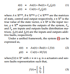
The goal is to estimate fu and fy as soon as possible such that, the monitored data are quickly corrected and at the same time the closed loop control system is able to correct the fault. Consequently, it is possible to prevent that the system is positioned outside the desired operating point or worse, become unstable.
Output observers
For fault detection and isolation (FDI) purposes, the estimation of all states is not required, it is sufficient to estimate of the output variables. For this reason, an output observer is appropriate for FDI [8]. The dynamic of this observer (Fig. 1) is,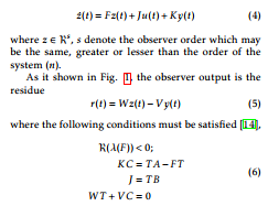
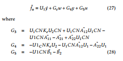
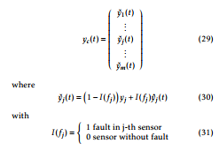
In order to isolate faults, a set of structural or directional residues is designed using this approach. Thus, the design of a structural residue set for sensor faults is straightforward. For example, if the output vector y = (y1,…,ym) is rewritten as
(y1,.,yi−1,yi+1,..,ym), the residue will be insensitive to the fault of the i −th sensor.
Contrary to the above, to isolate faults in the actuators through structural residues is not straightforward, but can be solved by means of unknown input observers (UIO).
2.2 Unknown input observers
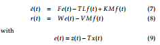
This subsection is based on the work of Hou and Muller [7] who proposed to design an observer whose¨ dimension is (n − q) for the purpose of detecting additive actuator faults. To do this, consider the LTI system (1) where A,B,C,Fu are constant matrices with appropriated dimensions. Furthermore, assume that m ≥ q and, without loss of generality, rank(Fu) = q and rank(C) = m.
Under this assumption, it is possible to choose a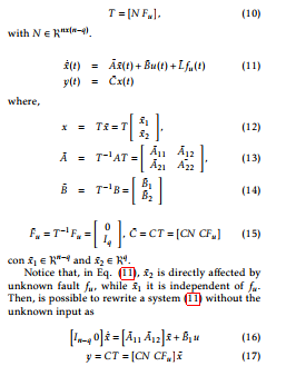
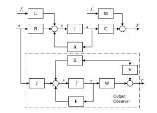
Figure 1: Process and output observer.
Assuming that x¯2 can be obtained from y, the Eq. (16) can be written as a conventional linear system. Indeed, if the matrix [CFu] is of full column rank, there exist a non-singular matrix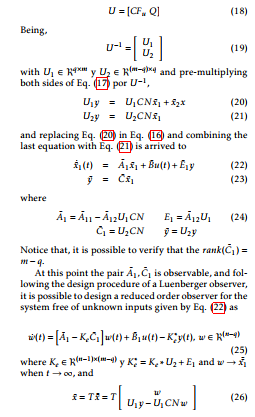
2.3 Observer banks
Figure 2 shows how to implement output and unknown input observer banks to estimate the residues according to the description in the previous two subsections.
3 Fault-tolerant control
The sensor and actuator faults do not impact in a system in the same way. Consequently, the solution for these two types of faults is different.
Fiqure 3 shows the FTC strategy based on [22] and [19] here implemented. Notice that, the detection, isolation and estimation consist in analyzing the results of each residue generator to decide if sensor or actuator is failing.
3.1 Design of FTC system for sensor faults
measurement and, the control loop is automatically reconfigured.When a particular sensor fault takes place, a free faults estimation of this particular sensor from observer bank is used, and this signal is feedback. That is, the estimated output variable is considered as good input observer (UIO) bank.
The estimation of j-th damaged sensor yˆj is obtained from an observer which is designed to be insensitive to fault of this j-th sensor. Consequently, the output vector used to implement the control law is
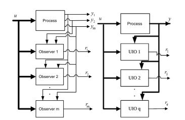
Figure 2: Observer Banks. (a) Output observer (OO) bank for all inputs and outputs except one.(b) Unknown output variable is considered as good input observer (UIO) bank.
3.2 Design of FTC system for actuator faults
When a fault in an actuator is detected, the control action is compensated by adding to manipulated variable whose value is proportional to the fault in order to minimize the impact.
In this work, a compensation to the control law proposed by [12] is added. Thus, under fault representation presented in Eq. (2 ), it is propose to add uacc to the nominal control action.
Therefore, when in a particular instant (tf ind) an actuator fault is detected, the control signal is corrected as follows:![]()
According to this new control law (Eq. (32)), the system described in state space given by Eq. (2) becomes, x˙(t) = Ax(t)+Bu(t)+Buacc +Lf u(t) (33)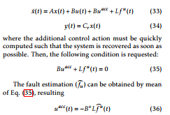
) where B+ is the pseudo-inverse matrix of the matrix B. This compensation control law is represented in Fig. (3) within the module denoted acomodation and estimation module.
4 Detecting faults in a CSTR
In order to analyze the system performance with the proposed observer banks above, it is proposed to simulate faults in a CSTR control system. The behavior of the system under actuator and sensor faults was simulated according to the classic non-linear model ([21, 9, 1, among others]) with the parameters suggested by [11].
4.1 CSTR non-linear model
Consider a CSTR represented in Fig. 4, where an irreversible exothermic chemical reaction A→B occurs. This reaction takes place in a cylindrical stirred tank
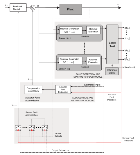
Figure 3: Scheme of a fault tolerant control system including detection and diagnostic module.
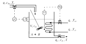
Figure 4: CSTR control schemes.
with a total capacity of Vmax = 120 l and a transversal section A = 0.2m2. The principal parameter values are summarized in Table 1.
The complete model (37) can be written according to a non-linear differential and algebraic equation set as follows: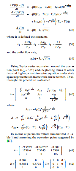
Finally, according to Fig. 4, the control system has two PI controllers, where the control variables are the temperature T and volume V , which will be controlled by the cooling flow qc and process flow rate q respectively.
4.2 Design of the observer banks
For this example, two observer bank were developed. One of them consist in three output observer to diagnose faults in the sensors of the volume, temperature and concentration, and the other one include two UIO to diagnose faults in the process and coolant flow rates.
4.3 Output observer design
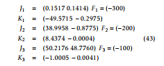
According to section 2.1, by means of Eqs. (6) the following vectors can be written:
|
Table 1: Nominal CSTR parameter values
Table 2: Signs of residues for different types of additive faults in the CSTR.
A
|
where the numerical subscript indicates the corresponding OO.
To interpret and isolate faults in the OO bank the isolation patterns are used. For these particular example, is applied a pattern as shown in Table 2.
For example, according to Table 2, if a fault increases the monitored temperature, a decrement of residue related to the reactant concentration (rcA) take place. Furthermore, an increment of temperature residue (rT ) and an invariant residue related to volume (rv) are observed. As a result of these behaviors, a temperature sensor fault can be inferred.
4.4 Unknown input observer design
According to section 2.2, the following matrices can be written: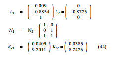
where L1 and L2 are the actuator fault vectors, N1 and N2 are proposals to satisfy Eq. (10), and Ke1 and Ke2 come from solving the equation of the observer (25).
4.5 Numerical simulation
The performance of FDI procedure here proposed by means of observer banks applied to additive faults are studied by means of numerical simulations.
|
Table 1: Nominal CSTR parameter values
Table 2: Signs of residues for different types of additive faults in the CSTR.
A
|
4.6 Temperature sensor fault
Firstly, set-point changes around the reactor operating point are proposed in order to show that the PI controllers allow tracking changes. In particular, the proposed changes are: the volume V = 110 L at t = 5 min and the temperature T = 435 ◦K at t = 15 min.
Figure 5 shows the reactor dynamic response when a 5 % degradation in the temperature sensor at t = 30 min takes place. According with Fig.6, without fault tolerant control, the control loop reduces the coolant flow qc to adjust the temperature of the reactor to the desired value according to an measured incorrect value, assuming that the reactor needs to accumulate more heat. Consequently, the actual temperature of the reactor is much higher at the end of the transient due to this unnecessary adjustment by the controller. However, this behavior does not take place if the FTC is implemented. Notice that, the same figure shows that when the sensor fault adaptation module (Fig. 3) is activated, the right signal is taken, therefore FTC system correction is involved and the reactor temperature value is maintained in T = 435 ◦K when steady state is reached.
Figure 7 shows how the residues (rT , rcA and rV ) indicate the presence of a fault in temperature sensor according to Table 2.
4.7 Volumen sensor fault
In this simulation is shown a change in the volume setpoint at t = 5 min from V = 100 L to V = 110 L, and then a 5% degradation in the volume sensor at t = 35 min.
Figure shows the system dynamic response without fault-tolerant control. The feedback signal from the volume sensor fails abruptly into −5%, monitoring a wrong value (V = 104.5 L). As a result of this fault, the control loop corrects the measurement error in order to maintain the level at 110 L. Thus, according to the fault assumed the monitored volume by the sensor suggests to the controller that is correcting properly.
Furthermore, in this figure can also be seen how the FTC reacts an instant later in which it follows that a fault has occurred, the sensor fault adaptation module switches the signal from the observer bank according to Fig. 3. Then, the controlled variable retrieves the set-point value while the measured signal from the sensor continues to the wrong value.
Notice that according to the introduced changes in temperature set-point in t = 15 min does not influence the dynamics of the reactor volume, this being consistent with the physics of the problem.
Figure 8 shows how the reactor temperature evolves for both volume set-point change and with volume sensor fault. Notice that when a volume setpoint change is introduced, a change in the reactor temperature is observed, forcing the temperature control loop to correct it (t = 5 min). Then, in the instant t = 35 min, the temperature corrections are made by the control loop. Figure 8 shows this corrections with and without FTC.
Figure 9 shows the dynamic response of temperature and the manipulated coolant flow for the problem with and without FTC, for the time interval between t = 30 min and t = 50 min. Based on the dynamic response without FTC it is possible to conclude
Figure 5: Actual CSTR temperature without FTC, measured temperature in the CSTR, set-point and temperature with FTC. Notice that the following changes was implemented: (1) a set-point change in the reactor volumen at t = 5 min, (2) a set-point change in the CSTR temperature at t = 15 min and, (3) a 5 % degradation in the temperature measuring element at t = 30 min.
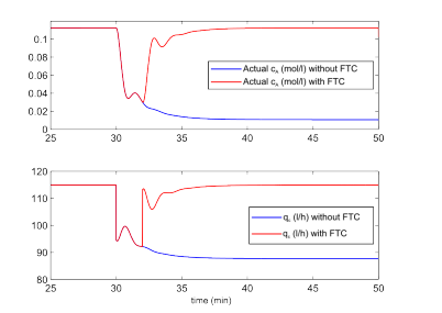
Figure 6: (a) Dynamic response of reactant concentration (cA) when a degradation of temperature sensor take place with and without FTC. (b) Dynamic response of manipulated variable (qc) with and without FTC.
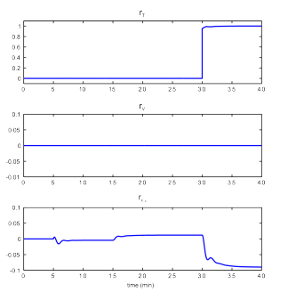
Figure 7: Residues of rT , rV and rcA to a fault in the temperature sensor.
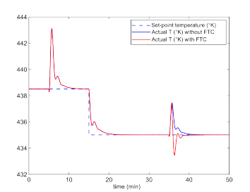
Figure 8: Actual and measured temperature and CSTR set-point. Notice that the following changes: (1) a set-point change in the volume at t = 5 min, (2) a set-point change in the CSTR temperature at t = 15 min and, (3) a 5 % degradation in the volume measuring element at t = 35 min.
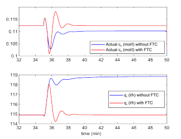
Figure 9: (a) Dynamic response of reactant concentration change (cA) when a fault in the volume sensor take place with and without FTC. (b) Dynamic response of manipulated variable (qc) with and without FTC.
that due to the actual volume of the reactor is not in the set-point value, it is necessary to increase the coolant flow to extract the heat required to bring the temperature back to the set-point.
5 Conclusions
In this paper, the design of an active fault tolerant control was presented, showing an adaptation to a fault in both an actuator and a sensor. To achieve this, two schemes that allow to compute residues through analytical redundancy was presented. The main proposal of this work is the use of observer banks to diagnostic sensor and actuator faults. In this context, output observers were used to detect sensor fault while an unknown input observer was used to identify manipulated variable fault.
This fault diagnosis strategy is applied to a CSTR, showing that the methodologies presented lead to satisfactory results. Furthermore, it is emphasized that the chosen example has specially interest in the chemical industry and, although there is many examples in the literature with non-linear systems using this methodology ([13, 8, among others]), but there is few references in FDI applied to CSTR [20, 3].
Finally, this work allows to understand even better the behavior of the CSTR when different faults taken placed.
Conflict of Interest
The authors declare no conflict of interest.
Acknowledgment
The authors would like to thank the financial support received by the Universidad Nacional del Litoral by means of its CAI+D program.
- E. J. Adam, Instrumentacioin y Control de Procesos. Notas de Clase, Ediciones UNL, 2nd edition, 2014.
- M. Blanke, M. Kinnaert, J. Lunze, and M. Staroswiecki, Diagnosis and Fault-Tolerant Control Systems, Springer, 2006.
- F. Caccavale, M. Iamarino, F. Pierri, and V. Tufano, Control and Monitoring of Chemical Batch Reactors, Springer, 2011.
- J. Chen, R. J. Patton, and H. Y. Zhang, “Design of unknown input observers and robust fault detection filters” Int. Journal of Control, 63(1), 85–105, 1996.
- P. M. Frank, “Fault diagnosis in dynamic system using analytical and knowledge-based redundancy – a survey and some new results” Automatica, 26(3), 459–474, 1990.
- J. Gertler, Fault detection and diagnosis in engineering systems, Marcel Dekker, Inc., 1998.
- M. Hou and P. C. Muller, “Design of observers for linear systems with unknown inputs” IEEE Trans. On Automatic Control, 37(6), 871–875, 1992.
- R. Isermann, Fault-Diagnosis System, Springer, 2006.
- W. Luyben, Process Modeling, Simulation and Control for Chemical Engineers, Mc Graw Hill, 1990.
- M. Mahmoud, J. Jiang, J. Lunze, and Y. Zhang, Active Fault Tolerant Control, Springer, 2003.
- J. D. Morningred, B. E. Paden, D. E. Seborg, and D. A. Mellichamp, “An adaptive nonlinear predictive controller” Proc. Amer. Contr.Conf., 2, 1614–1619, 1990.
- H. Noura, D. Sauter, F. Hamelin, and D. Theilliol, “Fault-tolerant control in dinamic systems: Application to a winding” IEEE Control Systems Magazine machine, 20(1), 33–49, 2000.
- H. Noura, D. Theilliol, J.C. Ponsart, and A. Chamseddine, Fault-Tolerant Control Systems, Springer, 2009.
- J. O’Reilly, Observers for Linear Systems, Academic Press, 1983.
- R. J. Patton and J. Chen, “Observer-based fault detectiona and isolation: Robustness and applications”, Control Eng. Practice, 5(5), 671–682, 1997.
- M. F. Pico and E. J. Adam, Advantages in residual methods for fault detection and isolation problem: application in laboratory experimental dc-motor in XIV Reunio?n de trabajo en Procesamiento de la Informacion y Control, RPIC 2011, Oro Verde, Argentina, 2011.
- M. F. Pico and E. J. Adam, Comparing fault detection and isolation methods applied to a laboratory experimental servomotor, CAIP 2011. X Cong. Interam. de Computacin Aplicada a la Industria de Procesos, Girona, Espaa, 2011.
- M. F. Pico and E. J. Adam, Control tolerante a fallas en un sistema de tanques aplicando redundancia analtica en el diagnstico de fallas, CIETA 2012. IX Cong. Int. Electrnica y Tecnologas de Avanzada, Pamplona, Colombia, 2012.
- M. F. Pico, “Dise ´ no de Controladores Tolerante a Fallas Aplicados a Procesos de la Industria Quımica”, Mag. Thesis, Univeridad Nacional del Litoral, 2015.
- O. A. Z. Sotomayor and D. Odloak, “Observerbased fault diagnosis un chemical plants”, Chemical Engineering Journal, 112:93–108, 2005.
- G. Stephanopoulos, Chemical Process Control, Prentice Hall, 1984.
- D. Theilliol, H. Noura and J.C. Ponsart, “Fault diagnosis and accommodation of a three-tank system based on analytical redundancy”, 41(3), 365–382, 2002.