1 Introduction

This paper is an extension of work originally presented in IEEE 11^th ICSC [1].

The task of capturing emotional meaning from audio structure while disregarding trivial or irrelevant information is a complex process that cannot be inferred using low-level acoustics. Recent advances in research on sound dynamics have shown that nonlinear phenomena exist in complex audio signals [2, 3, 4, 5, 6]. Such complex information is shaped in the nonlinear dynamical structure of audio content that is brought together by repeating patterns evolving in a temporal order. Nonlinear dynamics analysis consists of a set of methods that unravel these fine-grained patterns, and study their role in conveying meaningcarry perceptual meaning [8]. As a consequence recent studies were successful at applying methods of nonlinear dynamics to capture voice pathologies in speech signals [9, 3, 4, 10], recognize environmental sounds [11, 12] and discriminate between different singing styles [2]. Despite these advances, very few researches have applied nonlinear dynamics for modeling emotion in audio signals. In [6], measures of the geometrical properties of the phase space reconstruction are employed to recognize affect in speech; in [13], recurrence properties of the vowel accurately describe the dynamic behaviour of six basic emotions.

In our former work [1], we proposed a novel learning framework of affective auditory scene analysis us-

ing a recently developed method of non-linear dynamic signal analysis, the Variable Markov Oracle (VMO), that finds the best audio structure representation in terms of the symbolized recurring patterns, while preserving their temporal order. We obtained symbolic recurrence quantification analysis (RQA) measures without reconstructing the phase space with embedding. Our contribution over previous recurrence analysis methods is that our model explored the dynamics of the most informative recurrent patterns in the signal, by means of symbolic RQA features. We showed that measures of periodicity and complexity derived from our model are relevant for the characterization of affect in auditory scenes, and that they perform better than state-of-the-art methods relying on low-level acoustic features.

In this paper we contribute to the ongoing research on affective semantics from sound by proposing a new set of symbolic dynamical invariants computed from the VMO. After the symbolization step, we propose a novel method of computing symbolic dynamical invariants from the symbolized sequences of the time series, after performing an embedding step. The invariants are: the correlation dimension (D2), correlation entropy (K2) and the Lyapunov Exponent (LE). In literature, the correlation dimension and Lyapunov Exponent have been successful in discriminating voice quality as well as in characterizing pathologies in voice [14, 9]. Furthermore, D2 and K2 are effective in the detection of emotion in speech [3, 4]. In the music domain, LE and D2 were used to characterize the clarinet tone [15], however rare are the literatures that investigate the potential of dynamical invariants in characterizing emotion in music.

The contribution of this paper is a novel method of nonlinear dynamics that derives symbolic dynamical measures from an adaptive time series symbolization method (VMO), with and without phase space reconstruction. First, it derives symbolic RQA measures from a symbolization of the signal’s feature frames without embedding [1]. Second, it estimates symbolic dynamical invariants from the symbolized time series after embedding. Then we estimate our symbolic dynamical measures for the logistic map and show that they are in agreement with known methods from literature. Finally we test the performance of our symbolic complexity measures in predicting emotion by performing classification tasks on four types of sound stimuli. The advantage of our symbolic complexity measures is that first they quantify the dynamics of the most meaningful recurring patterns in the signal; second, their number is determined and hence we don’t have to address the problem of the dimensionality of the dataset, therefore no feature selection methods are employed; third we show that they are efficient in recognizing emotions across four types of stimuli, which suggests that their performance does not depend on the type of sound under study.

2          Theoretical Background

2.1         Nonlinear Time Series Analysis

Nonlinear time series analysis (NLTSA) consists of a set of methods that characterize dynamical information from time-ordered values in a dataset. It is based on the fact that the real underlying dynamical state of a complex system is often unknown, and that all the information needed to determine the future behaviour of the system’s state is independent of its past, and can be predicted based on knowledge of the present state, which is the observable measured by the time series.

In order to learn about the underlying dynamics of time-ordered data such as audio signals, it is necessary to reconstruct the phase space.

Phase Space Reconstruction The states of dynamical systems change in time, and their time evolution is defined geometrically in the shape of trajectories that belong to a phase space known as strange attractor.

In practice, we do not have a full knowledge of the dynamical system in order to reconstruct its phase space. But we do have a time-discrete measurement of one observable, which results in a scalar and discrete time series, that is used to reconstruct the original system’s dynamics, through the reconstruction of its phase space via embedding. The embedding theorems guarantee that for noise-free data, there is a dimension m such that the embedded vectors are equivalent to the original phase space vectors [16].

To reconstruct the phase space of a system from a time series, the Takens’ embedding theorem is used [17] and the framework is the following [18]:

Let x(t) be a trajectory of a dynamical system and s(t) = s(x(t)) the result of a scalar measurement on it. Then a delay reconstruction with time delay τ and embedding dimension m is given by:

               s(t) = (s(t − (m − 1)τ),s(t − (m − 2)τ),…,s(t))          (1)

Embedding parameters One of the main challenges of the delay-coordinate embedding theorem, is choosing appropriate values of dimension m and time lag τ [16].

Several methods exist that derive m and τ but we are naming the most widely used ones in literature. First τ is estimated: if τ is very small, consecutive elements of the delay vectors will highly correspond, and all the vectors will be clustered around the main diagonal, unless m is very large. If τ is very large, consecutive elements are independent, and the points will fill a large space in the phase space [16]. Two functions can be used to determine τ: the first zero of the autocorrelation function of the time series and the first minimum of the mutual information function (FMMI). In this work we use the FMMI.

Once τ is chosen, the next step is to estimate the embedding dimension m. If m is too large, the embedded data will be redundant, which will confuse the performance of prediction algorithms. Two widely known methods can be used: the false-nearest neighbour algorithm (FNN) [19] and the ‘asymptotic invariant approach’. The FNN method is used in this work since it is the most widely used one, and m is chosen where the number of false neighbours drops to zero.

The resulting phase space with dimension m is equivalent to the attractor in the original phase space with dimension d, if m ≤ 2d +1. In general we don’t know what the value of d is, but using the FNN method, m is guaranteed to fulfil that requirement.

2.2         Recurrence Plots

Recurrence is a fundamental property of most dynamical systems. In fact it is due to the systems’ recurrence to former states that we know how to predict the future state of the system. Recurrence takes place in the system’s phase space, and the tool that measures it is called a recurrence plot (RP) [20].

Given a trajectory x~_i ∈ _R^d in a d-dimensional phase space of a dynamical system, the RP is a twodimensional visualization of the square recurrence matrix of the embedded time series defined by:

                Rm,εi,j = Θ(ε −   x~i − x~j   ),     i,j = 1,…,N               (2)

where x~_i and x~_j are phase space trajectories in an m-dimensional phase space, N is the number of measured points in a trajectory, ε is a threshold distance, Θ(.) the Heaviside function such that: Θ(x) = 0 if x < 0 and Θ(x) = 1 otherwise, and k.k is some appropriate choice of a norm, such as the L₂-norm, otherwise known as the Euclidean distance. Both axes of the RP are time axes. The dots or pixels located at (i,j) and (j,i) on the RP are black if the distance between points x_i and x_j in the phase space fall inside a ball or threshold corridor of radius ε, the threshold distance [21, 22]. In this case, the black points refer to recurring states also termed ε-recurrent states since they occur in an ε-neighbourhood. The ε-recurrent states are represented by the relation[20]:

                                   x~i ≈ x~j ⇐⇒ Ri,j ≡ 1.                              (3)

The dots are white if R_i,j ≡ 0. The RP always displays a main black diagonal line called the line of identity (LOI), since R_i,i ≡ 1 by definition. For more in-depth description of the RP properties, the reader is referred to [20].

2.3         Recurrence Quantification Analysis

In order to derive meaning from the structures of the RP, various complexity measures are computed that quantify those structures. Such quantification is important since it will be employed to characterize the dynamical information and to perform predictions. These statistical measures are known as Recurrence Quantification Analysis (RQA) and are based on the density of recurrence points, the diagonal and vertical line structures in the RP [21, 23, 24]. RQA can be applied to non-stationary processes in continuous or discrete time series. For example, the metric determinism can discriminate signals from noise, and is valuable in pattern mining and classification tasks.

2.3.1     Measures based on the density of recurrence points

Given an RP thresholded at ε (Eq. 2), the Recurrence Rate (RR) measures the density of recurrence points in the RP:

N

1 X

                                   RR = N2            Ri,j                                                 (4)

i,j=1

The RR measure corresponds to the correlation sum (D2) measure, but D2 excludes the main diagonal line (LOI):

N

                                                 1           X

                               D2 = − 1)     R_i,j                                        (5)

N(N

i,j=1

j,i

2.3.2         Diagonal lines based measures

Given the histogram P (l) of diagonal lines of length l, the following measures are computed:

Determinism (DET ) is the percentage of points in diagonal line of at least length l = l_min, i.e. the ratio of recurrence points in the diagonals to all recurrence points, and is a measure of the predictability of the system. Processes with chaotic behaviour cause none or very short diagonals. Deterministic processes cause longer diagonals and less isolated recurrence points.

^PNl=l^min lP (l)

                                     DET = _PNl=1lP (l)                                   (6)

The average length of diagonal line length L is the average time during which two segments of a trajectory are close to each other, and it refers to the mean prediction time. The length l of diagonal lines refer to the number l of time steps during which a segment of the trajectory is close to another segment of the trajectory at a different time. Therefore the diagonal lines are related to the divergence of the trajectory segments.

^PNl=lmin lP (l)

                                       L = _PNl=lmin P (l)                                    (7)

Then the length L_max of the longest diagonal line in the RP excluding LOI is derived:

                                   Lmax = max({li}Ni=1l )                               (8)

And the inverse of L_max indicates the divergence (DIV ) of the phase space trajectory. The faster the trajectory segments diverge, the diagonal lines will be shorter, and the value of DIV will be higher:

1

                                          DIV =                                      (9)

Lmax

The next measure is the Shannon entropy of diagonal line length distribution in the RP (S_RP ), which is the probability p(l) = P (l)/N_l to find a diagonal line of exactly length l in the RP. It is a measure of complexity in the RP in terms of the diagonal lines, such that, for uncorrelated noise the value of S_RP will be small, which indicates a low complexity. It is defined as:

N

X

                                S_RP = −             p(l) ln p(l)                        (10)

l=lmin

The RAT IO is a measure that uncovers transitions in the system’s dynamics:

DET

                                       RAT IO =                                 (11)

RR

2.3.3         Vertical lines based measures

Measures based on vertical structures in the RP uncover chaos-chaos transitions [20] in a dynamical system that are not found using diagonal line based measures. These are laminarity and trapping time.

The laminarity (LAM) refers to the occurrence of laminar states in the system independently of their lengths. If the RP contains less vertical lines and more single recurrence points, then the value of LAM will be low. Its definition is analogous to the definition of DET for vertical lines of minimal length v = v_min.

PN= vP (v) v vmin

                                   LAM = _PNv=1vP (v)                               (12)

The trapping time measure (T T ) is the average length of vertical lines, and estimates the mean time that the system’s state will be trapeed:

^PNv=v^min vP (v)

                                    T T = _PNv=vmin P (v)                              (13)

3          Our Approach

One key concern when using RPs is finding the threshold to make sure that the RP exhibits enough recurrence points. Another difficulty to address is the length of the sequence used to generate the RP. This is considered as a second embedding step that is different from the phase space embedding, however in traditional RP construction methods these two steps are indistinguishable, as the RP is constructed first and then the recurring patterns are found by looking for diagonal lines.

In this work we propose a novel method that does not require a phase space reconstruction with embedding. This is done using the Variable Markov Oracle (VMO) [25], a suffix automaton that reduces a multivariate time series down to a symbolic sequence while retaining the recurring sub-sequences. Accordingly, we consider recurrences of symbolic sequences without a need to estimate a threshold, since this step is implicitly done during the symbolization, based on a mutual information criterion that estimates the optimal threshold in terms of maximizing Information Rate (IR) [26]. IR considers the mutual information between past and present in a signal. In the next section we describe this approach.

In a first phase, we estimate symbolic RQA from the symbolic RPs generated from the VMO without embedding. In a second phase, we estimate symbolic dynamical invariants from the VMO generated symbolic recurrences, after applying an embedding.

3.1         The Variable Markov Model

The Variable Markov Oracle (VMO) [25] is a suffix tree data structure that is derived from Factor Oracle (FO) [27, 28] as well as Audio Oracle (AO) [29].

FO is a suffix automaton that finds factors (repeated substrings) in a word (or sequence of symbols), as well as patterns (repeated suffixes) [27]. It has been employed mainly for optimal string matching algorithms, such as biosequence pattern matching. Assayag et al. 2004 showed how the FO can be adapted to learn symbolic musical sequences and generate symbolic musical improvisations in real-time [28].

AO is an extension of FO for audio signals, that is independent of the audio feature representation. AO extends the applications of FO to multivariate time series such as an audio signal sampled at discrete times. Based on a distance measure, the AO structure finds and links all the possible combinations of audio sub-

clips that are similar. AO has been successfully applied to audio generation.

3.1.1        VMO Construction

VMO inherits the strengths of both FO and AO. The important improvement over its predecessors, is that VMO assigns symbols to the signal frames connected by suffix links during AO construction: it accepts a signal O as input, outputs the oracle structure, and keeps track of the sequence of assigned labels Q = q₁,…,q_N as well as a list of pointers to their corresponding observations O = O[1],…,O[N]. As such VMO performs a symbolization of a signal’s time series by storing the information regarding the repeated substrings via the suffix links created during AO construction and upgrades AO by assigning labels to the frames connected by suffix links.

The notations of the forward and suffix links remain the same as in FO construction. The detailed algorithm is found in [30, 25].

As mentioned earlier, a similarity threshold θ is introduced to determine if a signal sample O[i] is similar to another sample O[j].

In order to find the best symbolization of the signal, different VMO models can be created with different θ values. There is a tradeoff to consider when choosing θ values. If θ is very low, every frame will be different than every other frame, and VMO assigns a different symbol to each frame in O. If θ is very high, frames that are different are considered similar, and the same symbol is assigned to every frame in O. In both cases no structure in the time series can be captured by VMO.

Hence θ should be determined before VMO construction. Dubnov et al. 2011 showed that the value of θ can be resolved by computing the Information Rate (IR) over candidate θ values [31]. The optimal θ value is the one that yields a highest IR value.

Information Rate IR is an information theoretic metric that measures the information content of a time series.

Let x₁^N = x₁,x₂,…,x_N be a time series x with N observations, where H(x) = −^PP (x)log₂P (x) is the entropy of x, then the definition of IR is [32]:

                         IR(x₁ⁿ⁻¹,x_n) = H(x_n) − H(x_n|x₁ⁿ⁻¹)                  (14)

And it is approximated by replacing the entropy terms in equation 14 by a complexity measure C associated with a compression algorithm [32]. The complexity measure is the number of bits used to compress x_n independently using the past observations ^x₁n−1:

1. IR) (15)

Compror is a lossless compression algorithm based on FO and the length of the longest repeated suffix link (lrs). Details on Compror as well as on the method of combining Compror with AO and IR are found in

[33]

IR is the mutual information between past and present observation in a signal O[t] and is maximized when there is balance between variation and repetition in the symbolized signal. This means that a VMO with a higher IR value captures more of the repeating patterns than a VMO with a lower IR value [32]. Figure 1 shows two oracle structures obtained with two extreme θ values. Figure 2 visualizes the sum of IR values versus different values of θ.

3.2         Symbolic Recurrence Plots from VMO

From the generated VMO-symbolized time series, we obtain the symbolic RP (RP_S hereafter), plotted from the binary self-similarity matrix. The index of a suffix link is a point on the RP_S and a repeated sequence is detected as a line since it includes repetitions of length 1, 2, up to the longest repeated length. This makes VMO effectively find a repetition for variable length non-uniform embedding.

We redefine the symbolic RP_S obtained from the optimal VMO model of the signal’s time series:

Ri,jM = Θ(θ − d(σqi ,σqj )) i,j = 1,…,N Such that:	(16)
 1        if d(σqi ,σqj )is ≤ θ   σM,θ =  Ri,j                   0 otherwise  	(17)

              ^{σ     ,θ}

Where N is the number of states considered, σ_M refers to the M^th symbolized substring, Θ is the Heaviside step function (i.e. Θ(x) = 0 if x < 0, and Θ(x) = 1 otherwise). θ is a threshold distance, and d(σ_qi ,σ_qj ) is a distance metric between pairs of symbolized substrings q_i at t = i and q_j at t = j.

3.3         Feature Extraction

In our experiments, we derive two sets of complexity features.

Symbolic RQA measures In the first phase we estimate symbolic RQA measures (RQA_S hereafter). Standard ways to consider similarity in audio signals is through time-frequency representation. In a preprocessing stage, the time series is transformed into a constant-Q transform (CQT) feature vector. CQT is a logarithmic spacing of filter center frequencies versus bandwidths, that represents the audio signal in a form that approximates human auditory analysis. Then the CQT feature vector is passed as input to the VMO constuction algorithm, that generates several symbolizations of the features in terms of their recurrence properties. by means of IR, the optimal threshold θ is evaluated to obtain the optimal VMO symbolization model M_S. Then the symbolic RP_S is generated from the self-similarity matrix obtained from the longest repeated substrings (LRS) of M_S. Then RQA_S estimates are obtained. Although standard RQA metrics are not invariants, in our case, since their estimation is independent of embedding, our RQA_S can be considered as invariants.

Symbolic Dynamical Invariants In the second phase we estimate symbolic dynamical invariants: the correlation dimension (D2), correlation entropy (K2) and the Lyapunov Exponent (LE).

Given a one-dimensional time series obtained from an audio signal, first we embed it using Takens’ time-delay embedding method. The dimension m is determined by the false-nearest neighbour algorithm, and the value is chosen where the false nearest neighbours are zero. The value of the time delay τ is defined by the first minimum of the mutual information function. Next, we symbolize it with VMO, and select M_S by means of IR. Then from the selected VMO model we obtain a representation of the LRS found in the series. From this representation we proceed to extract D2, K2 and LE. The framework is depicted in figure

3.

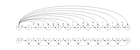Figure 1: Two oracle structures. The top oracle has a very low θ value. The bottom oracle has a very high θ value [30]

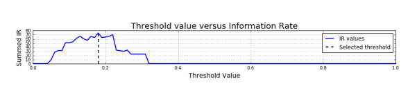Figure 2: IR values on vertical axis and on horizontal axis. The solid curve in blue shows the relations between the two measures and the dashed black line indicates the selected θ by locating the maximal IR value. [32]

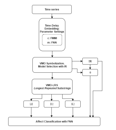Figure 3: Dynamical Invariants extraction framework

Normally, in order to derive the LE using Rosenstein’s algorithm or Eckmann’s algorithm, either algorithm operates directly on the time series after embedding, and then computes the LE. In our approach we obtain our symbolic invariants from the LRS of the optimal VMO model M_S. This is a novel aspect where we obtain symbolic dynamical invariants that describe the dynamical behaviour of only the most meaningful recurrences found in the series.

Before employing the dynamical invariants in emotion prediction tasks, we first probe to what extent our estimates are in agreement with known methods by illustrating their application to the logistic map. Then we question their role in discriminating emotion in voice, auditory scenes, instrumental music as well as in film music.

Correlation Dimension The correlation dimension (D2) is a geometric measure that tells how complex are the dynamics of the system: a more complex system has a higher dimension, which in is estimated from the symbolic recurrence plot. D2 estimates the complexity of the dynamics: a higher D2 indicates a more complex system’s dynamics. D2_S is computed from the symbolic RP_S by the correlation sum [20]:

N

1              X

                D2_S = N(N ₋ 1) Θ(θ − d(σ_qi ,σ_qj ))         (18)

i,j=1

j,i

Correlation Entropy The correlation entropy (K2) also known as 2^nd order Renyi entropy quantifies the´ loss of information in time, in a dynamic system. It is estimated from the symbolic RP_S as:

                                        K2_S = −ln(D2_S)                                 (19)

Lyapunov Exponent Lyapunov exponents (LE) estimate the amount of chaos in a dynamical system by quantifying the exponential divergence of initially close phase-space trajectories. A system with one or more positive LEs is defined to be chaotic.

4          Example Application

In this section we illustrate the application of the RQA_S as well as the symbolic dynamical invariants for synthetic examples of the logistic map. Logistic map is a well known model that exhibits different dynamic properties as a function of a single parameter, and allows comparing standard non-linear dynamic information measures with the data analysis methods we develop here. The logistic map model allows us to investigate some intriguing computational properties of sequences that happen at the onset of chaos.

4.1         Symbolic RQA_S for the logistic map

Mathematically, the equation of the logistic map is defined as:

                                       x_i+1 = ax_i(1 − x_i)                                (20)

where x_i is a real number between zero and one and a is a positive constant. We generate multiple time series from the logistic map and define the control parameter r ∈ [3.5,4], with ∆r = 0.0005, so that for each r we have a separate time series T of length 1000. The values of the parameters are set in order to compare the results with [20] and accordingly, we embed the time series with dimension m = 3 and time delay τ = 1.

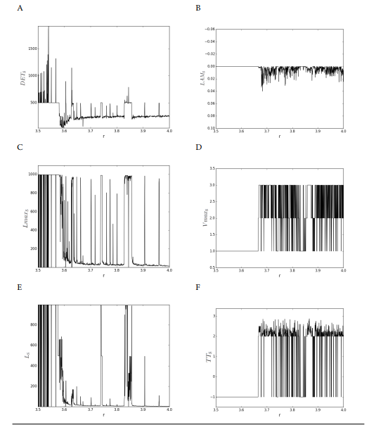Figure 4 shows plots of our VMO-derived RQA_S measures. A comparison of the plots below is made with similar plots in [20] derived directly from the time series after embedding.

Plots (A), (C), (E) of figure 4 show the measures DET_S, Lmax_S and L_S respectively that are based on the diagonal lines. They have similar maximas that indicate the periodic-chaos/chaos-periodic transitions. Lmax_S detects all such transitions, but DET_S and L_S do not find them all.

Similarly, the chaos-chaos transitions to the laminar states are depicted by the measures based on the vertical structures, shown in plots (B), (D), (F): LAM_S, T T_S and V max_S. The difference between LAM_S and V max_S is that LAM_S only measures the amount of

laminar states, while V max_S estimates the maximum duration of the laminar states. The lines in V max_S plot show significant drops within periodic windows, indicating that the chaos-order transitions are also identified. This is in agreement with [20] who states that RQA measures are able to identify bifurcation points. However the LAM_S plot shows a different structure, it displays minimas or drops that correspond to the chaos-chaos transitions, while in the referenced work the LAM plot displays maximas or peaks at the same locations. This may be due to the fact that our LAM_S is derived from a symbolic representation of the series rather than the data itself. However as in the referenced paper, LAM_S is different from the other two vertical-based measures V max_S and T T_S, in that it does not peak at inner crises, possibly because it is more robust against noise in the data. Finally similarly to the method in [20], with our symbolization method a 1000 data points are enough to derive the RP-based measures.

4.2         Symbolic dynamical invariants for the logistic map

To test the suitability of our symbolic complexity measures, we compute them for the logistic map. For each of LE, D2, K2, IR as well as θ, there is one value per time series.

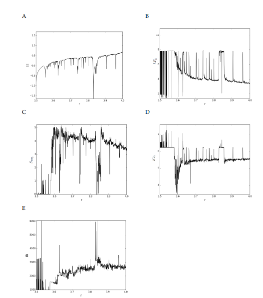Figure 5 portrays plots of the LE computed directly from the time series after embedding, the Shannon entropy (S_RPS) estimated from the RP_S, the symbolic LE_S and K2_S. The plots are commented in subsection 4.3.

Figure 4: RQA_S from the RP_S of the logistic map: r ∈ [3.5,4.0], ∆r = 0.0005 and T = 1000. (A) Determinism. (B) Maximal diagonal line length. (C) Average diagonal line length. (D) Laminarity. (E) Maximal vertical line length. (F) Trapping time.

The formal relationship between the correlation entropy K2 and the Lyapunov Exponents LE is [20]:

X

                                           K₂ ≤          λ_i                                                     (21)

λ_i>0

where λ_i denote the Lyapunov exponents. From Eq.(21) one sees that K2 is a lower bound for the sum of the positive Lyapunov exponents.

4.3         Qualitative Comparison of Dynamical Invariants

There are different dynamical regimes and transitions that occur between the values in the range of r of the logistic map. They appear in the form of accumulation points, periodic and chaotic states, band merging points, period doublings and various order-chaos, chaos-order as well as chaos-chaos transitions [34, 20].

In [35], authors applied various measures to derive statistical meaning from the graphical structures of symbolic recurrence plots. One such measure is the Shannon entropy of diagonal line length distribution in the RP (S_RPS).

The Shannon entropy is a measure of the complexity of the RP, such that for uncorrelated noise it takes a small value, which indicates a low complexity [20]. However it is not a dynamical invariant [36].

According to Eckmann et al. 1987, the diagonal line lengths on RPs are related to the inverse of the largest LE [37]. This is true for some cases despite the fact that empirical studies have shown that S_RPS is capable of identifying dynamical transitions, and therefore should grow as the system’s complexity grows.

[38].

Since the Shannon entropy quantifies the complexity of the dynamical system being studied, it is expected that its values increase when the system develops, that is when it varies from non-chaotic to chaotic regime [38]. Hence it is expected to be positively correlated with the LE, rather than negatively correlated. And within periodic windows, the entropy should considerably decrease.

Therefore in a recent work, [39] has proposed another estimation of the Shannon entropy from RPs from the relative frequency of the occurrence of the diagonal segments of nonrecurrent points formed by white dots, that are a signature of complexity within the data. In this case a one-to-one correspondence was seen between the new Shannon entropy estimate and the positive LE. That is, the Shannon entropy increased as the bifurcation parameter of the logistic equation increased, as illustrated in the plots found in [39]. However, [38] claim that the definition of the entropy from the white nonrecurrent dots does not solve the problem of the negative correlation between the entropy and the positive LE.

Here we compute the positive LE from the logistic map time series, after embedding and symbolization with VMO. The LE is computed from the VMOderived LRS, and the Shannon entropy is estimated from the VMO-derived symbolic RP_S.

Figure 5 (A) shows the plot of the LE obtained from the time series of the logistic map. Plot (C) displays the Shannon entropy S_RPS estimated from the black diagonal lines of the symbolic recurrence plot. The S_RPS plot detects the chaos-chaos transitions as well as the periodic-chaos and chaos-periodic transitions. The plot shows that the S_RPS correlates positively with the LE rather than with its inverse. We note though that for r ∈ [3.9,4.0] the values of the entropy seems to slightly decrease with the chaotic behaviour of LE. Further investigation is needed to understand this behaviour, that seems to correlate with the inverse of LE for that particular region of r.

It is clear that with our method, while maintaining the computation of the entropy from the black recurrence dots of the symbolic RP_S generated from the LRS of the symbolized time series, we obtain an estimate of the diagonal lines entropy that correlates positively with the Lyapunov exponents plot, with the exception of the region of r ∈ [3.9,4.0].

Plot (B) illustrates the LE_S obtained from the VMO-derived LRS. Plot (D) is the K2 plot derived from the RP_S and shows that the K2 plot is a lower bound of the LE_S plot. This verifies the relation expressed in Eq. 21, where K2 is defined as being a lower bound on the sum of the positive LEs.

Plot (E) displays the IR values that correspond to the optimal VMO model for each time series generated from the logistic map. By contrasting it with plot (A) of figure 4, we notice that the IR plot correlates positively to the determinism measure. Both show maximas or peaks at the chaos-order transitions. Additionally, IR captures the chaos-chaos transitions as well.

5          Model of Affect

Model of Affect. Affect can be described with basic emotional categories or emotional dimensions. We use categorical representations of Russel’s twodimensional model of valence and arousal (VA) described by pleasant-unpleasant for V, and awake-tired for A [40].

Stimuli. Four databases are used for experimental validation of the proposed symbolic dynamical features. The International Affective Digitized Sounds (IADS-2) [41] consists of a set of standardized, affective environmental sounds that span a broad range of semantic categories, and are rated on the twodimensional model of VA.

The Montreal Affective Voices (MAV) [42] consist of 90 nonverbal affect bursts, enacted by 10 different actors in the following 8 categorical emotions: anger, disgust, feat, pain, sadness, surprise, happiness and pleasure, in addition to the neutral expression. The durations of the vocalizations vary between 0.385 to 2.229 seconds sampled at 44100 Hz. In order to perform a comparative analysis with different databases and to ensure consistency in the affective annotations,

Figure 5: Dynamical Invariants of logistic map: r ∈ [3.5,4.0], ∆r = 0.0005. (A) LE from the time series. (B) LE_S from LRS. (C) Shannon entropy from RP_S. (D) K2_S from RP_S. (E) Information rate from RP_S.

the emotional categories of MAV sounds were mapped on the VA model described by: pleasant-unpleasant (V) and awake-tired (A).

The Musical Emotional Bursts (MEB) [43] consist of 80 short instrumental musical clips, played using the clarinet and the violin, in the following 3 categorical emotions: happiness, sadness and fear, plus the neutral expression. The mean duration of the MEB clips is of 1.6 seconds. The discrete emotions were mapped on the VA model.

The Film Music Excerpts (FME) [44] consist of 360 musical excerpts at 44100 Hz sampling rate, annotated on the VA dimensional model of emotions described with: high valence, low valence, high energy, low energy. The FME is designed to provide musical stimuli that allow a systematic comparison of the perceived emotions in music.

Dataset. Two datasets are evaluated: the symbolic RQA_S measures for the IADS, MAV, MEB and FME stimuli, and symbolic dynamical invariants for the IADS, MAV and FME stimuli.

Classification Model. In this work we use a feedforward artificial neural net (ANN) [45]. The feedforward ANN is chosen for its simplicity and suitability for the problem studied. The network has one hidden layer and one output layer. It was trained with the Levenberg- Marquardt as well as the scale conjugate gradient backpropagation learning algorithms, and the validation was performed using the mean squared error function (MSE).

6          Experiments

The experimental work as well as the results obtained are described in this section.

6.1         Experimental work

For the computation of the RQA_S dataset, the CQT is obtained at 44100 Hz sampling rate, hop length of 512 and 84 bins. Then we apply the symbolization process and estimate the RQA_S. For the computation of the dynamical invariants, the time series is embedded first and then we apply the symbolization. The datasets are normalized before training so that column features are scaled to have standard deviation 1, and centered to have mean 0.

Classification. The dataset is divided into 70% training, 15% validation and 15% testing. The classification tasks are conducted in a multi-class oneversus-all fashion whereby each of the six affective sub-dimensions is in turn considered as positive and negative class. The final results are then averaged to get the classifier’s performance on VA. The Neural Network Toolbox in MATLAB is used. No feature selection was made prior to classification.

Performance evaluation. If the dataset is too small or biased, over-fitting can occur. Therefore in addition to the MSE function, we applied the Adaptive Synthetic Sampling (ADASYN) algorithm to rebalance the datasets. The classifier’s performance is evaluated before and after dataset rebalancing, using a combination of performance metrics taken from the confusion matrix. These are: accuracy (ACC), precision, recall, F1-measure, F2-measure, area under the receiver operating characteristic curve (AUC), as well as Cohen’s Kappa. Accuracy and precision are highly sensitive to data imbalance therefore three additional measures are computed: Cohen’s Kappa (κ), F1-measure and F2-measure.

6.2         Results

Classification performance

In order to evaluate the generalizability of our features, we tested them on four different types of stimuli.

The classification performance rates of the RQA_S measures are reported in tables 1 to 5, and performance rates of the dynamical invariants are in tables 6 and 8.

In table 1, the prediction accuracies on VA are

(74%, 90%) respectively for the auditory scenes (IADS). Comparing to other existing work, in [46] a classification task was evaluated for the IADS database using a set of 101 acoustic features, and achieved a performance of less than 50% accuracy. We note some poor metrics values such as κ is very low for the arousal dimension indicating an agreement close to chance level; AUC is 0.66 for valence. However the values of F₁, F₂, precision and recall are fairly high. These results could be consolidated or checked if the same tests are repeated with a much larger dataset.

In tables 2 and 3 high prediction accuracies of (97%, 90%) and (81%, 90%) are attained respectively on VA for the musical clips. The values of the remaining metrics are higher for the violin music than for the clarinet music. Although in both cases κ > 0.40 for both VA which shows an agreement above chance level between observed and predicted values.

Table 4 shows a success rate of (79%, 93%) on VA for the MAV dataset using RQA_S. This rate is verified with the values of the remaining metrics which are fairly high: both F₁ and F₂ are > 0.70, κ > 0.40, and the AUC is close to 1 for arousal and 0.79 on valence.

In table 5, the classification results on the FME dataset using the RQA_S metrics are of (65%, 77%) on VA. This shows that the RQA_S do not capture well valence in the film music excerpts. Further investigations are needed in this respect, to determine what is impacting the differences in the recognition rates between the short music clips and the short film music excerpts.

The classification success rates using the dynamical invariants achieve (72%, 82%) for IADS (table 6), (69%, 73%) for FME (table 7) and (84%, 91%) for MAV

(table 4). The invariants perform well for IADS and MAV, however they have a rather low rate for FME, although they perform better than RQA_S on valence.

In [47], an emotion classification task is made on

Table 1: RQA_S performance measures for IADS on VA

Affect	ACC	PPV	TPR	F1	F2	κ	AUC
Valence	0.74	0.93	0.73	0.82	0.76	0.17	0.66
Arousal	0.90	1.00	0.90	0.94	0.92	0.06	0.72

Table 2: RQA_S performance measures for Violin music on VA

Affect	ACC	PPV	TPR	F1	F2	κ	AUC
Valence	0.97	0.95	0.98	0.96	0.97	0.93	0.98
Arousal	0.90	0.73	1.00	0.83	0.92	0.76	0.92

Table 3: RQA_S performance measures for Clarinet music on VA

Affect	ACC	PPV	TPR	F1	F2	κ	AUC
Valence	0.81	0.75	0.71	0.73	0.72	0.56	0.85
Arousal	0.90	0.83	0.89	0.86	0.88	0.78	0.95

Table 4: RQA_S performance measures for MAV on VA

Affect	ACC	PPV	TPR	F1	F2	κ	AUC
Valence	0.79	0.78	0.77	0.74	0.75	0.47	0.79
Arousal	0.93	0.78	0.81	0.79	0.80	0.75	0.96

Table 5: RQA_S performance measures for FME on VA

Affect	ACC	PPV	TPR	F1	F2	κ	AUC
Valence	0.65	0.60	0.87	0.71	0.80	0.30	0.71
Arousal	0.77	0.87	0.46	0.60	0.51	0.47	0.83

Table 6: Dynamical invariants performance measures on IADS

Affect	ACC	PPV	TPR	F1	F2	κ	AUC
Valence	0.72	0.91	0.71	0.79	0.74	0.14	0.64
Arousal	0.82	0.78	0.76	0.75	0.75	0.09	0.61

Table 7: Dynamical invariants performance measures for FME on VA

Affect	ACC	PPV	TPR	F1	F2	κ	AUC
Valence	0.69	0.69	0.70	0.69	0.70	0.39	0.75
Arousal	0.73	0.72	0.46	0.56	0.50	0.38	0.79

Table 8: Dynamical invariants performance measures for MAV on VA

Affect	ACC	PPV	TPR	F1	F2	κ	AUC
Valence	0.84	0.72	0.80	0.75	0.78	0.59	0.91
Arousal	0.91	0.61	0.90	0.72	0.82	0.45	0.91

the same FME stimuli, using 200 acoustic features and five emotional categories: anger, fear, happiness, sadness and tenderness. The recognition rates using support vector machines (SVM) are: 65%, 67%, 59%, 69% and 67% for the five emotions respectively. Although in our case we did not use discrete emotions but the VA model, however with only five nonlinear dynamical features our recognition rates are (69%, 73%) and using our RQA_S the rates are (65%, 77%).

7          Conclusive Remarks and Discussion

In this work we proposed a novel method to estimate complexity measures from the symbolic RP_S of the VMO symbolized time series of audio signals. The symbolic RQA_S measures were estimated without phase space reconstruction. The symbolic dynamical invariants were estimated after embedding. We estimated our dynamical measures for the symbolized time series of the logistic map and through a qualitative analysis of the respective plots, we showed that our symbolic measures are in agreement with the same measures obtained using different methods in literature. Furthermore, we estimated the symbolic Shannon entropy S_RPS of the RP diagonal lines from the LRS of the optimal VMO model, and showed that it correlates positively with the Lyapunov exponents except for the region r ∈ [3.9,4.0].

In order to evaluate the performance of our symbolic dynamical measures in characterizing affect in various sounds, we conducted classification tasks on four types of stimuli. High emotion recognition rates were achieved for the IADS, MAV and MEB datasets for both sets of symbolic measures. This highlights the powerful performance of the measures in emotion recognition independently of the type of stimuli and shows that they generalize well across different types of stimuli. Furthermore it encourages future work to test the features in large scale tasks to determine if they can gain consensus as a general-purpose feature set.

However we obtained rather low recognition rates for film music excerpts on valence, and an average rate for arousal of 77% and 73%. Further work is needed to explore why both sets of complexity measures, the RQA_S as well as the dynamical invariants obtained in this work, achieve rather low recognition rates on film music excerpts, compared to the results obtained on the IADS, MAV as well as the music clips datasets. Obviously the dynamics differ across different sounds, but it would be interesting for future work to further investigate what particular aspects of the dynamics carry affective information. It would also be interesting to determine how such knowledge differs across different types of audio signals.

Conflict of Interest The authors declare no conflict of interest.

1. Pauline Mouawad and Shlomo Dubnov. Novel method of non-linear symbolic dynamics for semantic analysis of auditory scenes. In Semantic Computing (ICSC), 2017 IEEE 11th International Conference on, pages 433–438. IEEE, 2017.
2. Caitlin J Butte, Yu Zhang, Huangqiang Song, and Jack J Jiang. Perturbation and nonlinear dynamic analysis of different singing styles. J Voice, 23(6):647–652, 2009.
3. Patricia Henríquez, Jesús B Alonso, Miguel A Ferrer, Carlos M Travieso, and Juan R Orozco-Arroyave. Application of nonlinear dynamics characterization to emotional speech. In International Conference on Nonlinear Speech Processing, pages 127– 136. Springer, 2011.
4. Patricia Henríquez, Jesús B Alonso, Miguel A Ferrer, Carlos M Travieso, and Juan R Orozco-Arroyave. Nonlinear dynamics characterization of emotional speech. Neurocomputing, 132:126–135, 2014.
5. Hanspeter Herzel. Bifurcations and chaos in voice signals. Appl. Mech. Rev, 46(7):399–413, 1993.
6. Ali Shahzadi, Alireza Ahmadyfard, Ali Harimi, and Khasha-yar Yaghmaie. Speech emotion recognition using nonlinear dynamics features. Turk J Elec Eng & Comp Sci., 23(Sup. 1):2056–2073, 2015.
7. Peter beim Graben and Axel Hutt. Detecting recurrence domains of dynamical systems by symbolic dynamics. Phys. Rev. Lett., 110(15):154101, 2013.
8. Julyan HE Cartwright, Diego L González, and Oreste Piro. Pitch perception: A dynamical-systems perspective. Proceedings of the National Academy of Sciences, 98(9):4855–4859, 2001.
9. Patricia Henríquez, Jesús B Alonso, Miguel A Ferrer, Carlos M Travieso, Juan I Godino-Llorente, and Fernando Díazde María. Characterization of healthy and pathological voice through measures based on nonlinear dynamics. IEEE Trans. Audio, Speech, Language Process., 17(6):1186–1195, 2009.
10. C de A Washington, FM de Assis, BG Aguiar Neto, Silvana C Costa, and Vincius JD Vieira. Pathological voice classification based on recurrence quantification measures. 2012.
11. Gerard Roma, Waldo Nogueira, and Perfecto Herrera. Recurrence quantification analysis features for environmental sound recognition. In 2013 IEEE Workshop on Applications of Signal Processing to Audio and Acoustics, pages 1–4. IEEE, 2013.
12. Gerard Roma, Waldo Nogueira, Perfecto Herrera, and Roc de Boronat. Recurrence quantification analysis features for auditory scene classification. IEEE AASP Challenge: Detection and Classification of Acoustic Scenes and Events, Tech. Rep, 2013.
13. Angela Lombardi, Pietro Guccione, and Cataldo Guaragnella. Exploring recurrence properties of vowels for analysis of emotions in speech. Sensors & Transducers, 204(9):45, 2016.
14. Jesús B Alonso, Fernando Díazde María, Carlos M Travieso, and Miguel Angel Ferrer. Using nonlinear features for voice disorder detection. In ISCA tutorial and research workshop (ITRW) on non-linear speech processing, 2005.
15. Teresa D Wilson and Douglas H Keefe. Characterizing the clarinet tone: Measurements of lyapunov exponents, correlation dimension, and unsteadiness. The Journal of the Acoustical Society of America, 104(1):550–561, 1998.
16. Holger Kantz and Thomas Schreiber. Nonlinear time series analysis, volume 7. Cambridge university press, 2004.
17. Floris Takens. Detecting strange attractors in turbulence. In Dynamical systems and turbulence, Warwick 1980, pages 366– 381. Springer, 1981.
18. Thomas Schreiber. Interdisciplinary application of nonlinear time series methods. Phys. Rep., 308(1):1–64, 1999.
19. Matthew B Kennel, Reggie Brown, and Henry DI Abarbanel. Determining embedding dimension for phase-space reconstruction using a geometrical construction. Physical review A, 45(6):3403, 1992.
20. Norbert Marwan, M Carmen Romano, Marco Thiel, and Jürgen Kurths. Recurrence plots for the analysis of complex systems. Physics reports, 438(5):237–329, 2007.
21. Elizabeth Bradley and Folger Kantz. Nonlinear time-series analysis revisited. Chaos, 25(9):097610, 2015.
22. Jerome Rolink, Martin Kutz, Pedro Fonseca, Xi Long, Berno Misgeld, and Stefen Leonhardt. Recurrence quantification analysis across sleep stages. BIOMED SIGNAL PROCES, 20:107–116, 2015.
23. David Schultz, Stephan Spiegel, Norbert Marwan, and Sahin Albayrak. Approximation of diagonal line based measures in recurrence quantification analysis. Phys. Lett. A, 379(14):997– 1011, 2015.
24. Charles L Webber, Norbert Marwan, Angelo Facchini, and Alessandro Giuliani. Simpler methods do it better: success of recurrence quantification analysis as a general purpose data analysis tool. Phys. Lett. A, 373(41):3753–3756, 2009.
25. Cheng-i Wang and Shlomo Dubnov. The variable markov oracle: Algorithms for human gesture applications. IEEE Multi-Media, 22(4):52–67, 2015.
26. Shlomo Dubnov. Spectral anticipations. Comput. Music J., 30(2):63–83, 2006.
27. Cyril Allauzen, Maxime Crochemore, and Mathieu Raffinot. Factor oracle: A new structure for pattern matching. In International Conference on Current Trends in Theory and Practice of Computer Science, pages 295–310. Springer, 1999.
28. Gérard Assayag and Shlomo Dubnov. Using factor oracles for machine improvisation. Soft Comp., 8(9):604–610, 2004.
29. Shlomo Dubnov, Gerard Assayag, and Arshia Cont. Audio oracle: A new algorithm for fast learning of audio structures. In Proceedings of International Computer Music Conference (ICMC). ICMA, 2007.
30. Cheng-i Wang and Shlomo Dubnov. Guided music synthesis with variable markov oracle. In The 3rd International Workshop on Musical Metacreation, 10th Artificial Intelligence and Interactive Digital Entertainment Conference, 2014.
31. Shlomo Dubnov, Gérard Assayag, and Arshia Cont. Audio oracle analysis of musical information rate. In Semantic Computing (ICSC), 2011 Fifth IEEE International Conference on, pages 567–571. IEEE, 2011.
32. Cheng-i Wang and Shlomo Dubnov. Pattern discovery from audio recordings by variable markov oracle: A music information dynamics approach. In Proc IEEE Int Conf Acoust Speech Signal Process., pages 683–687. IEEE, 2015.
33. Arnaud Lefebvre and Thierry Lecroq. Compror: on-line loss-less data compression with a factor oracle. Inform. Process. Lett., 83(1):1–6, 2002.
34. Pierre Collet and J-P Eckmann. Iterated maps on the interval as dynamical systems. Springer Science & Business Media, 2009.
35. LL Trulla, A Giuliani, JP Zbilut, and CL Webber. Recurrence quantification analysis of the logistic equation with transients. Phys. Lett. A, 223(4):255–260, 1996.
36. H Rabarimanantsoa, L Achour, C Letellier, A Cuvelier, and J-F Muir. Recurrence plots and shannon entropy for a dynamical analysis of asynchronisms in noninvasive mechanical ventilation. Chaos, 17(1):013115, 2007.
37. J-P Eckmann, S Oliffison Kamphorst, and David Ruelle. Recur-rence plots of dynamical systems. EPL (Europhysics Letters), 4(9):973, 1987.
38. Deniz Eroglu, Thomas K DM Peron, Nobert Marwan, Francisco A Rodrigues, Luciano da F Costa, Michael Sebek, István Z Kiss, and Jürgen Kurths. Entropy of weighted recurrence plots. Physical Review E, 90(4):042919, 2014.
39. Christophe Letellier. Estimating the shannon entropy: recur-rence plots versus symbolic dynamics. Physical review letters, 96(25):254102, 2006.
40. Ulrich Schimmack and Alexander Grob. Dimensional models of core affect: A quantitative comparison by means of structural equation modeling. Eur. J. Pers., 14(4):325–345, 2000.
41. Margaret M Bradley and Peter J Lang. The international affective digitized sounds (; iads-2): Affective ratings of sounds and instruction manual. University of Florida, Gainesville, FL, Tech. Rep. B-3, 2007.
42. Pascal Belin, Sarah Fillion-Bilodeau, and Frédéric Gosselin. The montreal affective voices: a validated set of nonverbal affect bursts for research on auditory affective processing. Behav Res Methods., 40(2):531–539, 2008.
43. S Paquette, I Peretz, and P Belin. The musical emotional bursts: a validated set of musical affect bursts to investigate auditory affective processing. Frontiers in Psychology, 4(509):1–7, 2013.
44. Tuomas Eerola and Jonna K Vuoskoski. A comparison of the discrete and dimensional models of emotion in music. Psychol. Music, 39(1):18–49, 2011.
45. Philip J Drew and John RT Monson. Artificial neural net-works. Surgery, 127(1):3–11, 2000.
46. Konstantinos Drossos, Andreas Floros, and Nikolaos-Grigorios Kanellopoulos. Affective acoustic ecology: towards emotionally enhanced sound events. In Proceedings of the 7th Audio Mostly Conference: A Conference on Interaction with Sound, pages 109–116. ACM, 2012.
47. Cyril Laurier, Olivier Lartillot, Tuomas Eerola, and Petri Toiviainen. Exploring relationships between audio features and emotion in music. In ESCOM 2009: 7th Triennial Conference of European Society for the Cognitive Sciences of Music, 2009.

(Click to view)

(Click to view)